Download
1 / 19
190 likes | 313 Vues
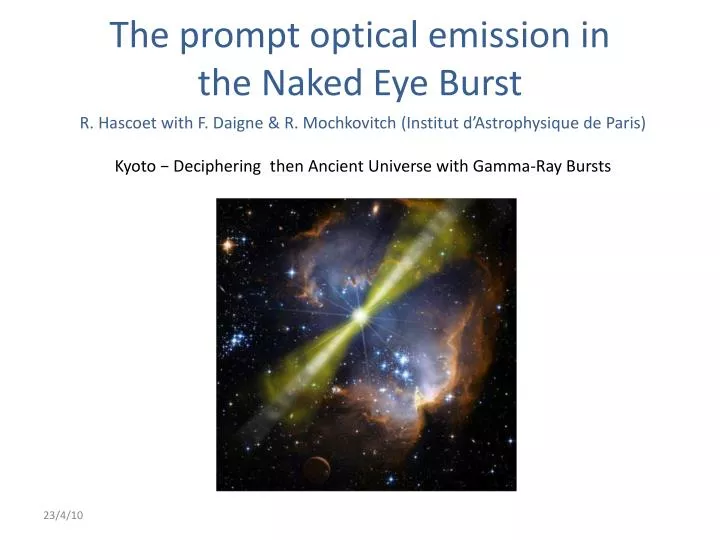
R. Hascoet with F. Daigne & R. Mochkovitch ( Institut d’Astrophysique de Paris) Kyoto − Deciphering then Ancient Universe with Gamma-Ray Bursts. The prompt optical emission in the Naked Eye Burst. Modeling the « Naked Eye Burst ». ( Racusin et al. 2008 ).

E N D
R. Hascoet with F. Daigne & R. Mochkovitch (Institutd’Astrophysique de Paris)Kyoto − DecipheringthenAncientUniversewithGamma-RayBursts The prompt optical emission in the Naked Eye Burst
Modeling the « Naked Eye Burst » (Racusin et al. 2008) Observations : a cosmological naked eye burst- For the first time, optical light curve during the whole prompt emission high temporal resolution. - huge radiated energy : Eg,iso = 1.3×1054 erg (20 keV – 7 MeV) - redshift :z = 0.937- V magnitude peak : mV,max = 5.3 (bright as 107 galaxies) Huge optical brightness – big challenge for the different models – Light curves (gamma & optical) g-ray spectrum optical ✕
Different scenarios already proposed Scenario 1 (single zone) : Synchrotron-Self Compton radiation from a single electron population • Optical : synchrotron • Gamma : first IC scattering on the synchrotron photons(Racusin et al. 2008)(Kumar & Panaitescu 2008) • (Kumar & Narayan 2009) ✕ No self-abs Self-abs Scenario 2 (single zone) : Synchrotron radiation from two electron populations • Optical : synchrotron – mildly relativistic electron pop. • Gamma : synchrotron – highly relativistic electron pop. ✕ No self-abs Self-abs These two scenarios face big problems : energy crisis, ….(Zou, Piran & Sari 2008)
Scenario 3 : Huge optical brightness due to a highly variable jet Log(R) [m] Internal Shock model • Variability during the ejection : “fast” shells catch up with “slow” shells (G ≈ 100) • Shocks : magnetic field amplification particle acceleration (relativistic electrons) • Radiation (g-rays) from the electrons : Synchrotron – IC • We use a multi-shell model as proposed by Daigne & Mochkovitch 1998 Huge optical brightness due to a highly variable jet ( Lorentz Factor : Gmax/Gmin≈ 5 - 10) (see also Yu, Wang, Dai 2009) Synchrotron radiation from shock-accelerated electrons in multi-shocked regions - gamma component : violent shocks - optical component : mild shocks
Huge optical brightness due to a highly variable jetInternal Shock model framework violent shockcontribution Proposed scenario : 1 electron population in multiple regions – Synchrotron emission - optical component : mild shocks - gamma component : violent shocks mild shock contribution ✕ No self-abs Self-abs initial profile Characteristic photon energy vs. radius Spectrum – Asymptotic Synch.(Sari, Piran & Narayan 1998) Ekin,iso = 5⋅1055 erg ee = 1/3 eB = 1/3 z = 10-2 Optical light curve Gamma light curve Ekin,iso = 5⋅1055 erg ee = 1/3 eB = 1/3 z = 10-2 Ekin,iso = 5⋅1055 erg ee = 1/3 eB = 1/3 z = 10-2 Ekin,iso = 5⋅1055 erg ee = 1/3 eB = 1/3 z = 10-2 Ekin,iso = 5⋅1055 erg ee = 1/3 eB = 1/3 z = 10-2 Ekin,iso = 5⋅1055 erg ee = 1/3 eB = 1/3 z = 10-2
Huge optical brightness due to a highly variable jetInternal Shock model framework violent shockcontribution Proposed scenario : 1 electron population in multiple regions – Synchrotron emission - optical component : mild shocks - gamma component : violent shocks mild shock contribution ✕ initial profile Characteristic photon energy vs. radius Spectrum – Ad hoc Ekin,iso = 5⋅1055 erg ee = 1/3 eB = 1/3 z = 10-2 Optical light curve Gamma light curve
(gamma & optical) Summary The Naked Eye Burst : why is it so bright in the optical domain ? • The high optical brightness of the Naked Eye Burst is very challenging for GRB models. • Proposed scenario : the initial outflow is highly variable. A potential problem : the shape of the gamma-ray spectrum in some cases. Due to a high dispersion in the characteristic energies of the emitted photons Reproduced observational features (with a fair probability : Monte Carlo analysis) : • High optical flux : - mainly built up by the milder shocks • The optical light curve is less variable than the gamma-ray one : - G of the shocked material is smaller for mild shocks (Dtobs ≈ R/2G2c) • The optical light curve begins after the gamma-ray one : - the optical synchrotron emission of the shocks with smaller radii is self-absorbed • The optical light curve ends after the gamma-ray one : - same reason as for (2.) - late shocks enhance the delay, in some cases (Racusin et al. 2008) The precise predicted fraction of optically bright bursts depends on the unknown central engine exact properties
Statisticalapproach – Monte Carlo Simulation – the physics of the central engineisstillunclear – What is the probability of having a burst such as the “naked eye burst” ? Whatwouldbe the probability of an eventsuch as the NakedEyeBurst ? Gvalues are uniformly distributed between 200 or 800 G varies on timescales 0.5s andis forced to be either 200 or 800 (with equal probability) Series of 500 runs 66% cases brighter than GRB080319B Example of the − optical mean flux − N N Cumulative fraction 16% cases brighter than GRB080319B Cumulative fraction
Modeling Internal Shocks • Discretisation of the jet in N shells • Successive collisions between these shells mimic the propagation of shock waves • We follow the evolution of the physical conditions in shocked regions
Modeling Internal Shocks • Discretisation of the jet in N shells • Successive collisions between these shells mimic the propagation of shock waves • We follow the evolution of the physical conditions in shocked regions Shock2 Shock1
Modeling Internal Shocks • Discretisation of the jet in N shells • Successive collisions between these shells mimic the propagation of shock waves • We follow the evolution of the physical conditions in shocked regions Shock2 Shock1
Modeling Internal Shocks • Discretisation of the jet in N shells • Successive collisions between these shells mimic the propagation of shock waves • We follow the evolution of the physical conditions in shocked regions Shock2 Shock1
Modeling Internal Shocks • Discretisation of the jet in N shells • Successive collisions between these shells mimic the propagation of shock waves • We follow the evolution of the physical conditions in shocked regions Shock2 Shock1
Modeling Internal Shocks • Discretisation of the jet in N shells • Successive collisions between these shells mimic the propagation of shock waves • We follow the evolution of the physical conditions in shocked regions Shock2 Shock1
Modeling Internal Shocks • Discretisation of the jet in N shells • Successive collisions between these shells mimic the propagation of shock waves • We follow the evolution of the physical conditions in shocked regions Shock1
Modeling Internal Shocks • Discretisation of the jet in N shells • Successive collisions between these shells mimic the propagation of shock waves • We follow the evolution of the physical conditions in shocked regions Shock1
Modeling Internal Shocks • Discretisation of the jet in N shells • Successive collisions between these shells mimic the propagation of shock waves • We follow the evolution of the physical conditions in shocked regions Shock1
Modeling Internal Shocks • Discretisation of the jet in N shells • Successive collisions between these shells mimic the propagation of shock waves • We follow the evolution of the physical conditions in shocked regions Shock1
Modeling Internal Shocks • Discretisation of the jet in N shells • Successive collisions between these shells mimic the propagation of shock waves • We follow the evolution of the physical conditions in shocked regions