Splay Trees
Comp 750, Fall 2009. Splay Trees - 2. BST: Search. 44. 88. 17. 65. 97. 32. 28. 54. 82. 76. 29. 80. . . . . . . . . . . . . . . . . . . . . . . . . . . . . . . . . . . . . . Note: In the handout,sentinel leaf nodes areassumed.? tree with n keyshas 2n 1 nodes.. . . . . . Search(25). . . . . . S

Splay Trees
E N D
Presentation Transcript
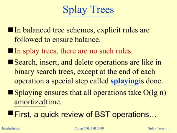
1. Comp 750, Fall 2009 Splay Trees - 1 Splay Trees In balanced tree schemes, explicit rules are followed to ensure balance.
In splay trees, there are no such rules.
Search, insert, and delete operations are like in binary search trees, except at the end of each operation a special step called splaying is done.
Splaying ensures that all operations take O(lg n) amortized time.
First, a quick review of BST operations�
2. Comp 750, Fall 2009 Splay Trees - 2 BST: Search
3. Comp 750, Fall 2009 Splay Trees - 3 BST: Insert
4. Comp 750, Fall 2009 Splay Trees - 4 BST: Delete
5. Comp 750, Fall 2009 Splay Trees - 5 BST: Delete
6. Comp 750, Fall 2009 Splay Trees - 6 BST: Delete
7. Comp 750, Fall 2009 Splay Trees - 7 BST: Delete
8. Comp 750, Fall 2009 Splay Trees - 8 Splaying In splay trees, after performing an ordinary BST Search, Insert, or Delete, a splay operation is performed on some node x (as described later).
The splay operation moves x to the root of the tree.
The splay operation consists of sub-operations called zig-zig, zig-zag, and zig.
9. Comp 750, Fall 2009 Splay Trees - 9 Zig-Zig
10. Comp 750, Fall 2009 Splay Trees - 10 Zig-Zag
11. Comp 750, Fall 2009 Splay Trees - 11 Zig
12. Comp 750, Fall 2009 Splay Trees - 12 Complete Example
13. Comp 750, Fall 2009 Splay Trees - 13 Complete Example
14. Comp 750, Fall 2009 Splay Trees - 14 Complete Example
15. Comp 750, Fall 2009 Splay Trees - 15 Complete Example
16. Comp 750, Fall 2009 Splay Trees - 16 Complete Example
17. Comp 750, Fall 2009 Splay Trees - 17 Complete Example
18. Comp 750, Fall 2009 Splay Trees - 18 Complete Example
19. Comp 750, Fall 2009 Splay Trees - 19 Complete Example
20. Result of splaying
The result is a binary tree, with the left subtree having all keys less than the root, and the right subtree having keys greater than the root.
Also, the final tree is �more balanced� than the original.
However, if an operation near the root is done, the tree can become less balanced. Comp 750, Fall 2009 Splay Trees - 20
21. Comp 750, Fall 2009 Splay Trees - 21 When to Splay Search:
Successful: Splay node where key was found.
Unsuccessful: Splay last-visited internal node (i.e., last node with a key).
Insert:
Splay newly added node.
Delete:
Splay parent of removed node (which is either the node with the deleted key or its successor).
Note: All operations run in O(h) time, for a tree of height h.
22. Comp 750, Fall 2009 Splay Trees - 22 Amortized Analysis Based on the Accounting Method (see Sec. 17.2 of CLRS).
Idea: When an operation�s amortized cost exceeds it actual cost, the difference is assigned to certain tree nodes as credit.
Credit is used to pay for subsequent operations whose amortized cost is less than their actual cost.
Most of our analysis will focus on splaying.
The BST operations will be easily dealt with at the end.
23. Comp 750, Fall 2009 Splay Trees - 23 Review: Accounting Method Stack Example:
Operations:
Push(S, x).
Pop(S).
Multipop(S, k): if stack has s items, pop off min(s, k) items.
24. Comp 750, Fall 2009 Splay Trees - 24 Accounting Method (Continued) We charge each operation an amortized cost.
Charge may be more or less than actual cost.
If more, then we have credit.
This credit can be used to pay for future operations whose amortized cost is less than their actual cost.
Require: For any sequence of operations, amortized cost upper bounds worst-case cost.
That is, we always have nonnegative credit.
25. Comp 750, Fall 2009 Splay Trees - 25 Accounting Method (Continued)
26. Comp 750, Fall 2009 Splay Trees - 26 Ranks T is a splay tree with n keys.
Definition: The size of node v in T, denoted n(v), is the number of nodes in the subtree rooted at v.
Note: The root is of size 2n+1.
Definition: The rank of v, denoted r(v), is lg(n(v)).
Note: The root has rank lg(2n+1).
Definition: r(T) = ?v?T r(v).
27. Meaning of Ranks The rank of a tree is a measure of how well balanced it is.
A well balanced tree has a low rank.
A badly balanced tree has a high rank.
The splaying operations tend to make the rank smaller, which balances the tree and makes other operations faster.
Some operations near the root may make the rank larger and slightly unbalance the tree.
Amortized analysis is used on splay trees, with the rank of the tree being the potential Comp 750, Fall 2009 Splay Trees - 27
28. Comp 750, Fall 2009 Splay Trees - 28 Credit Invariant We will define amortized costs so that the following invariant is maintained.
So, each operation�s amortized cost = its real cost + the total change in r(T) it causes (positive or negative).
Let Ri = op. i�s real cost and ?i = change in r(T) it causes. Total am. cost = ?i=1,�,n (Ri + ?i). Initial tree has rank 0 & final tree has non-neg. rank. So, ?i=1,�n ?i ? 0, which implies total am. cost ? total real cost.
29. Comp 750, Fall 2009 Splay Trees - 29 What�s Left? We want to show that the per-operation amortized cost is logarithmic.
To do this, we need to look at how BST operations and splay operations affect r(T).
We spend most of our time on splaying, and consider the specific BST operations later.
To analyze splaying, we first look at how r(T) changes as a result of a single substep, i.e., zig, zig-zig, or zig-zag.
Notation: Ranks before and after a substep are denoted r(v) and r?(v), respectively.
30. Comp 750, Fall 2009 Splay Trees - 30 Proposition 13.6
31. Comp 750, Fall 2009 Splay Trees - 31 Case 1: zig-zig
32. Comp 750, Fall 2009 Splay Trees - 32 Case 2: zig-zag
33. Comp 750, Fall 2009 Splay Trees - 33 Case 3: zig
34. Comp 750, Fall 2009 Splay Trees - 34 Proposition 13.7
35. Meaning of Proposition
If d is small (less than 3(r(t) ? r(x)) + 2) then the splay operation can increase r(t) and thus make the tree less balanced.
If d is larger than this, then the splay operation decreases r(t) and thus makes the tree better balanced.
Note that r(t) ? 3lg(2n + 1)
Comp 750, Fall 2009 Splay Trees - 35
36. Comp 750, Fall 2009 Splay Trees - 36 Amortized Costs As stated before, each operation�s amortized cost = its real cost + the total change in r(T) it causes, i.e., ?.
This ensures the Credit Invariant isn�t violated.
Real cost is d, so amortized cost is d + ?.
The real cost of d even includes the cost of binary tree operations such as searching.
Note: ? can be positive or negative (or zero).
If it�s positive, we�re overcharging.
If it�s negative, we�re undercharging.
37. Comp 750, Fall 2009 Splay Trees - 37 Another Look at ?
38. Unbalancing the Tree
In fact, a sequence of zig operations can result in a completely unbalanced linear tree. Then a search operation can take O(n) time, but this is OK because at least n operations have been performed up to this point. Comp 750, Fall 2009 Splay Trees - 38
39. Comp 750, Fall 2009 Splay Trees - 39 A Bound on Amortized Cost
40. Comp 750, Fall 2009 Splay Trees - 40 Finishing Up Until now, we�ve just focused on splaying costs.
We also need to ensure that BST operations can be charged in a way that maintains the Credit Invariant.
Three Cases:
Search: Not a problem � doesn�t change the tree.
Delete: Not a problem � removing a node can only decrease ranks, so existing credits are still fine.
Insert: As shown next, an Insert can cause r(T) to increase by up to lg(2n+3) + lg 3. Thus, the Credit Invariant can be maintained if Insert is assessed an O(lg n) charge.
41. Comp 750, Fall 2009 Splay Trees - 41 Insert
42. Comp 750, Fall 2009 Splay Trees - 42 Insert
43. Comp 750, Fall 2009 Splay Trees - 43 Proposition 13.8
44. Comp 750, Fall 2009 Splay Trees - 44 Proposition 13.9

