Download
1 / 27
280 likes | 656 Vues
Splay Trees and B-Trees. CSE 373 Data Structures Lecture 9. Readings. Reading Sections 4.5-4.7. Self adjusting Trees. Ordinary binary search trees have no balance conditions what you get from insertion order is it

E N D
Splay Trees and B-Trees CSE 373 Data Structures Lecture 9
Readings • Reading • Sections 4.5-4.7 Splay Trees and B-Trees - Lecture 9
Self adjusting Trees • Ordinary binary search trees have no balance conditions • what you get from insertion order is it • Balanced trees like AVL trees enforce a balance condition when nodes change • tree is always balanced after an insert or delete • Self-adjusting trees get reorganized over time as nodes are accessed • Tree adjusts after insert, delete, or find Splay Trees and B-Trees - Lecture 9
Splay Trees • Splay trees are tree structures that: • Are not perfectly balanced all the time • Data most recently accessed is near the root. (principle of locality; 80-20 “rule”) • The procedure: • After node X is accessed, perform “splaying” operations to bring X to the root of the tree. • Do this in a way that leaves the tree more balanced as a whole Splay Trees and B-Trees - Lecture 9
Splay Tree Terminology • Let X be a non-root node with 2 ancestors. • P is its parent node. • G is its grandparent node. G G G G P P P P X X X X Splay Trees and B-Trees - Lecture 9
Zig-Zig and Zig-Zag Parent and grandparentin same direction. Parent and grandparentin different directions. Zig-zig 4 G G 5 P 5 Zig-zag 1 P X 2 X Splay Trees and B-Trees - Lecture 9
Splay Tree Operations 1. Helpful if nodes contain a parent pointer. parent element right left 2. When X is accessed, apply one of six rotation routines. • Single Rotations (X has a P (the root) but no G) • ZigFromLeft, ZigFromRight • Double Rotations (X has both a P and a G) • ZigZigFromLeft, ZigZigFromRight • ZigZagFromLeft, ZigZagFromRight Splay Trees and B-Trees - Lecture 9
Zig at depth 1 (root) • “Zig” is just a single rotation, as in an AVL tree • Let R be the node that was accessed (e.g. using Find) • ZigFromLeft moves R to the top faster access next time root ZigFromLeft Splay Trees and B-Trees - Lecture 9
Zig at depth 1 • Suppose Q is now accessed using Find • ZigFromRight moves Q back to the top root ZigFromRight Splay Trees and B-Trees - Lecture 9
Zig-Zag operation • “Zig-Zag” consists of two rotations of the opposite direction (assume R is the node that was accessed) (ZigFromLeft) (ZigFromRight) ZigZagFromLeft Splay Trees and B-Trees - Lecture 9
Zig-Zig operation • “Zig-Zig” consists of two single rotations of the same direction (R is the node that was accessed) (ZigFromLeft) (ZigFromLeft) ZigZigFromLeft Splay Trees and B-Trees - Lecture 9
Decreasing depth - "autobalance" Find(T) Find(R) Splay Trees and B-Trees - Lecture 9
Splay Tree Insert and Delete • Insert x • Insert x as normal then splay x to root. • Delete x • Splay x to root and remove it. (note: the node does not have to be a leaf or single child node like in BST delete.) Two trees remain, right subtree and left subtree. • Splay the max in the left subtree to the root • Attach the right subtree to the new root of the left subtree. Splay Trees and B-Trees - Lecture 9
Example Insert • Inserting in order 1,2,3,…,8 • Without self-adjustment 1 O(n2) time for n Insert 2 3 4 5 6 7 8 Splay Trees and B-Trees - Lecture 9
With Self-Adjustment 1 2 3 1 ZigFromRight 1 2 2 1 3 2 ZigFromRight 2 1 3 1 Splay Trees and B-Trees - Lecture 9
With Self-Adjustment 3 4 4 2 4 ZigFromRight 3 1 2 1 Each Insert takes O(1) time therefore O(n) time for n Insert!! Splay Trees and B-Trees - Lecture 9
Example Deletion 10 splay (Zig-Zag) 8 5 15 5 10 13 20 15 2 8 2 6 9 13 20 6 9 Splay (zig) attach remove 6 5 10 5 10 15 15 2 6 9 2 9 13 20 13 20 Splay Trees and B-Trees - Lecture 9
Analysis of Splay Trees • Splay trees tend to be balanced • M operations takes time O(M log N) for M > N operations on N items. (proof is difficult) • Amortized O(log n) time. • Splay trees have good “locality” properties • Recently accessed items are near the root of the tree. • Items near an accessed one are pulled toward the root. Splay Trees and B-Trees - Lecture 9
13:- 17:- 6:11 6 7 8 11 12 3 4 13 14 17 18 Beyond Binary Search Trees: Multi-Way Trees • Example: B-tree of order 3 has 2 or 3 children per node • Search for 8 Splay Trees and B-Trees - Lecture 9
B-Trees B-Trees are multi-way search trees commonly used in database systems or other applications where data is stored externally on disks and keeping the tree shallow is important. A B-Tree of order M has the following properties: 1. The root is either a leaf or has between 2 and M children. 2. All nonleaf nodes (except the root) have between M/2 and M children. 3. All leaves are at the same depth. All data records are stored at the leaves. Internal nodes have “keys” guiding to the leaves. Leaves store between M/2 and M data records. Splay Trees and B-Trees - Lecture 9
ki k1 ki-1 kM-1 . . . . . . B-Tree Details Each (non-leaf) internal node of a B-tree has: • Between M/2 and M children. • up to M-1 keys k1 <k2 < ... <kM-1 Keys are ordered so that: k1 <k2 < ... <kM-1 Splay Trees and B-Trees - Lecture 9
k 1 Properties of B-Trees Children of each internal node are "between" the items in that node. Suppose subtree Ti is the ith child of the node: all keys in Ti must be between keys ki-1 and ki i.e. ki-1£ Ti < ki ki-1 is the smallest key in Ti All keys in first subtree T1 < k1 All keys in last subtree TM ³ kM-1 k k . . . k k k k . . . M-1 i-1 i i . . . . . . T T T T T T 1 1 i i M Splay Trees and B-Trees - Lecture 9
Example: Searching in B-trees • B-tree of order 3: also known as 2-3 tree (2 to 3 children) • Examples: Search for 9, 14, 12 • Note: If leaf nodes are connected as a Linked List, B-tree is called a B+ tree – Allows sorted list to be accessed easily 13:- - means empty slot 17:- 6:11 6 7 8 11 12 3 4 13 14 17 18 Splay Trees and B-Trees - Lecture 9
13:- 17:- 6:11 6 7 8 11 12 3 4 13 14 17 18 Inserting into B-Trees • Insert X: Do a Find on X and find appropriate leaf node • If leaf node is not full, fill in empty slot with X • E.g. Insert 5 • If leaf node is full, split leaf node and adjust parents up to root node • E.g. Insert 9 Splay Trees and B-Trees - Lecture 9
13:- 17:- 6:11 6 7 8 11 12 3 4 13 14 17 18 Deleting From B-Trees • Delete X : Do a find and remove from leaf • Leaf underflows – borrow from a neighbor • E.g. 11 • Leaf underflows and can’t borrow – merge nodes, delete parent • E.g. 17 Splay Trees and B-Trees - Lecture 9
Run Time Analysis of B-Tree Operations • For a B-Tree of order M • Each internal node has up to M-1 keys to search • Each internal node has between M/2 and M children • Depth of B-Tree storing N items is O(log M/2 N) • Find: Run time is: • O(log M) to binary search which branch to take at each node. But M is small compared to N. • Total time to find an item is O(depth*log M) = O(log N) Splay Trees and B-Trees - Lecture 9
Summary of Search Trees • Problem with Binary Search Trees: Must keep tree balanced to allow fast access to stored items • AVL trees: Insert/Delete operations keep tree balanced • Splay trees: Repeated Find operations produce balanced trees • Multi-way search trees (e.g. B-Trees): More than two children • per node allows shallow trees; all leaves are at the same depth • keeping tree balanced at all times Splay Trees and B-Trees - Lecture 9