Matrix Algebra
200 likes | 309 Vues
Learn the fundamentals of matrix algebra with this comprehensive guide featuring explanations, examples, and practical applications. Explore scalars, vectors, matrices, matrix operations, determinants, and more. Understand key concepts with visual aids and worked examples.

Matrix Algebra
E N D
Presentation Transcript
Matrix Algebra Methods for Dummies FIL January 25 2006 Jon Machtynger & Jen Marchant
Acknowledgements / Info • Mikkel Walletin’s (Excellent) slides • John Ashburner (GLM context) • Slides from SPM courses: http://www.fil.ion.ucl.ac.uk/spm/course/ • Good Web Guides • www.sosmath.com • http://mathworld.wolfram.com/LinearAlgebra.html • http://ceee.rice.edu/Books/LA/contents.html • http://archives.math.utk.edu/topics/linearAlgebra.html
2 3 Scalars, vectors and matrices • Scalar:Variable described by a single number – e.g. Image intensity (pixel value) • Vector: Variable described by magnitude and direction • Matrix: Rectangular array of scalars Square (3 x 3) Rectangular (3 x 2) d r c : rthrow, cthcolumn
Matlab notes ( ; End of matrix row ) A = [ 21 5 53 ; 5 34 12 ; 6 33 55 ; 74 27 3 ] To extract data: Matrix name( row, column ) Scalar Data Point A( 1 , 2 ) = 2 Row Vector A( 2 , : ) = [ 5 34 12 ] Column Vector A( : , 3 ) = [ 53 ; 12 ; 55 ; 3 ] Smaller Matrix A(2:4,1:2) = [ 5 34 ; 6 33 ; 74 27 ] Another Matrix A( 2:2:4 , 2:3 ) = [ 34 12 ; 27 3 ] Matrices • A matrix is defined by the number of Rows and the number of Columns. • An mxn matrix has mrows and ncolumns. A = 4x3 matrix • A square matrix of order n, is an nxn matrix.
Matrix addition Addition (matrix of same size) • Commutative: A+B=B+A • Associative: (A+B)+C=A+(B+C) Subtraction consider as the addition of a negative matrix
Matrix multiplication Constant (or Scalar) multiplication of a matrix: Matrix multiplication rule: When A is a mxn matrix & B is a kxl matrix, the multiplication of AB is only viable if n=k. The result will be an mxl matrix.
Jen’s way of visualising the multiplication Visualising multiplying A matrix = ( m x n ) B matrix = ( k x l ) A x B is only viable if k = n width of A = height of B Result Matrix = ( m x l )
Transposition column → row row →column Mrc = Mcr
Example Two vectors: Note: (1xn)(nx1) (1X1) Inner product = scalar Outer product = matrix Note: (nx1)(1xn) (nXn)
Worked example A In = A for a 3x3 matrix: Identity matrices • Is there a matrix which plays a similar role as the number 1 in number multiplication? Consider the nxnmatrix: • A square nxn matrix Ahas one • A In = InA = A • An nxm matrix A has two!! • InA = A & A Im = A
Inverse matrices • Definition. A matrix A is nonsingular or invertible if there exists a matrix B such that: worked example: • Notation. A common notation for the inverse of a matrix A is A-1. • The inverse matrix A-1 is unique when it exists. • If A is invertible, A-1 is also invertible A is the inverse matrix of A-1. • If A is an invertible matrix, then (AT)-1 = (A-1)T
- - - + + + Determinants • Determinant is a function: • Input is nxn matrix • Output is a real or a complex number called the determinant • In MATLAB • use the command det(A)" to compute the determinant of a given square matrix A • A matrix A has an inverse matrix A-1 if and only if det(A)≠0.
Matrix Inverse - Calculations Note: det(A)≠0 i.e. A general matrix can be inverted using methods such as the Gauss-Jordan elimination, Gaussian elimination or LU decomposition
Some Application Areas • Simultaneous Equations • Simple Neural Network • GLM
System of linear equations Resolving simultaneous equations can be applied using Matrices: • Multiply a row by a non-zero constant • Interchange two rows • Add a multiple of one row to another row Also known as Gaussian Elimination …
Simplistic Neural Network Weights learned in auto associative manner or given random values… O = output vector I = input vector W = weight matrix η = Learning rate d = Desired output t = time variable Given an input, provide an output… Over time, modify weight matrix to more appropriately reflect desired behaviour
Design Matrix = the betas (here : 1 to 9) data vector (Voxel) parameters design matrix error vector a m b3 b4 b5 b6 b7 b8 b9 = + × = + Y X b e
Design Matrix = the betas (here : 1 to 9) data vector (Voxel) parameters design matrix error vector a m b3 b4 b5 b6 b7 b8 b9 = + × = + Y X b e