Vegetation Indices
Vegetation Indices. Lecture 11 prepared by R. Lathrop 3/06. Remote Sensing of the Earth: Clues to a Living Planet. Remote sensing scientists measure the amount of energy in different spectral wavelengths reflected from the earth’s surface as one means of monitoring the earth’s biosphere.

Vegetation Indices
E N D
Presentation Transcript
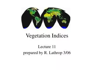
Vegetation Indices Lecture 11 prepared by R. Lathrop 3/06
Remote Sensing of the Earth: Clues to a Living Planet • Remote sensing scientists measure the amount of energy in different spectral wavelengths reflected from the earth’s surface as one means of monitoring the earth’s biosphere. • Where there are a lot of plants on the earth’s surface, less red and blue light is measured by the satellite sensor. Likewise, the more green plants, the more near infrared energy that is measured. • By combining measurements in the red and near-infrared wavelengths, scientists have devised a remotely sensed vegetation index or what is sometimes referred to as a ‘greenness index’. The more plants, the greener the earth, the higher the index.
Vegetation Indices • Linear combination of image bands used to extract information about vegetation: biomass, leaf area, productivity • Most vegetation indices (VI’s) based on the differential reflectances of healthy green vegetation, dead/senescent vegetation and soil in visible vs. near IR wavelengths
Photosynthetically Active Radiation • PAR : 0.40-0.70 um, portion of EMR absorbed by plant pigments and used in photosynthesis • APAR: PAR energy actually absorbed by a plant canopy • IPAR: intercepted PAR, probability that photons are intercepted by plant elements
How plant leaves reflect light Graphics from http://landsat7.usgs.gov/resources/remote_sensing/radiation.php
How plant leaves reflect light Blue & red light strongly absorbed by chlorophyll Sunlight B G R NIR NIR Incoming light Cross-section of leaf Reflected light NIR light scattered within leaf: some reflected back, some transmitted through Leaf Transmitted light
Reflectance from green plant leaves • Chlorophyll absorbs large % of red and blue for photosynthesis- and strongly reflects in green (.55um) • Peak reflectance in leaves in near infrared (.7-1.2um) up to 60% of infrared energy per leaf is scattered up or down due to cell wall size, shape, leaf condition (age, stress, disease), etc. • Reflectance in Mid IR (2-4um) influenced by water content-water absorbs IR energy, so live leaves reduce mid IR return
Sub-pixel Estimation N I R Re f l e c tance Spectral Feature Space Increasing Vegetation Example Pixel X proportions: IS: 50% Grass: 30% Trees: 20% Soil Line As green leaf area increases NIR increases red decreases Red Reflectance
Bi-directional reflectance efects • Lambertian surface: reflected energy is scattered equally in all directions; no direction bias = isotropic • Vegetation canopies are not Lambertian surfaces but rather demonstrate definite directional bias = anistropic • Aerial photos of tree canopies often exhibit the bi-directional reflectance differences as a result of the principal point perspective view • Tree crowns in the direction of incoming radiation expose their shady side to the image and those in the opposite direction show their illuminated sides.
Bidirectional Reflectance Distribution Function: BRDF • BRDF is the hemispherical distribution of reflectances for a feature as a function of illumination geometry • Bottom line: viewing and illumination angle are important; a nadir view of the same feature may record a different reflectance than a side view or look differently under different sun angles • Some sensors designed to provide different look angles at the same feature; e.g., a forward, nadir and backwards view • Once quantified, the BRDF can be used to correct for differential illumination effects
Measuring the BRDF: example Aircraft-mounted radiometer used to fly a closed circle and record reflectance of a site Note that the reflectance is not equally distributed across all directions Graphics from http://car.gsfc.nasa.gov/application_brdf.html
Simple method for correcting BR effect in aerial photographs • Adjust BR-affected brightness values of the aerial photographs (AP) with temporally concurrent but coarser scale imagery (e.g., Landsat TM) on a equivalent band-by-band basis • Normalize each pixel by multiplying by the ratio of mean TM over mean AP within a moving window centered on the AP pixel • APadj = TMwindow/APwindow * APorig • See Tuominen and Pekkarinen. 2004. RSE 89:72-82
Vegetation indices • Simple ratio: nir/red • Normalized Difference VI (NDVI): nir - red nir + red NDVI ranges from -1 to + 1 • Transformed VI to eliminate negative values: TVI : /NDVI + 0.5
Vegetation Indices: Issues • VI is a B&W image positively correlated with “greenness”, as NIR increases and red decreases, VI increases AVHRR Landsat TM
Vegetation Indices: Issues • Soil brightness variations complicating the VI response • Asymptotic relationship leading to loss in sensitivity at high vegetation amounts • Atmospheric interference, especially in the Red band. • Best practice is to convert the original DN values to radiance (preferably atmospherically corrected) or reflectance before computing the vegetation index
Vegetation Indices: Issues • Scaling: ratio of averages (NDVI of larger pixels; e.g., AVHRR pixels) is not the same as the average of the ratios (average NDVI of smaller pixels; e.g., Landsat TM) Example (sample area from Landsat TM: 30 m pixels vs. km2 composite) Ratio of averages: Mean red = 28 3 Mean NIR = 73 NDVI = (73-28)/(73+28) = 45/101 = 0.446 Average of ratios: NDVI = 0.416
Vegetation indices:PVI • Perpendicular VI determines a pixel’s orthogonal distance from the soil line in image feature space (X axis: red; Y axis: NIR) • The objective is to remove the effect of soil brightness and isolate reflectance changes due to vegetation only
Vegetation Indices:SAVI • Soil Adjusted Vegetation Index (SAVI) is a technique to minimize soil brightness influences. Involves shifting the origin of the nir-red feature space to account for 1st order soil-vegetation interactions and differential red & nir extinction through vegetation canopies • SAVI = (1+L) (nir-red) / (nir + red + L) Where L = 0 to 1. L = 1 for low veg density, L = 0.5 for intermed veg density L = 0.25 for high veg density From: Huete, A.R., 1988. A soil-adjusted vegetation index (SAVI), Rem. Sens. Environ. 25:295-309.
From: Huete, A.R., 1988. A soil-adjusted vegetation index (SAVI), Rem. Sens. Environ. 25:295-309.
Vegetation indices:MSAVI • Modified Soil Vegetation Index (MSAVI) employs a correction factor to reduce sensitivity to soil variation across a scene MSAVI0 = ((NIR – RED) (1 + L0)) / (NIR + RED +L0) MSAVI1 = ((NIR – RED) (2 - MSAVI0)) / NIR + RED +1 – MSAVI0 Must empirically determine L MSAVI2 = (2NIR + 1 – ((2NIR +1)2 – 8(NIR – RED)) -1/2 / 2
Vegetation indices: ARVI • Atmospherically Resistant Vegetation Index (ARVI) incorporates the blue channel to account for atmospheric scattering in the red channel by using the difference between the radiance in the red and blue channel • ARVI = (NIR – RB) / (NIR + RB) Where RB = Red – g (Blue – Red) Where Blue is Landsat TM band 1 ,visible blue wavelengths g = 1, unless the aerosol model is known a priori
Vegetation indices: EVI Enhanced Vegetation Index (EVI): developed to optimize the vegetation signal with improved sensitivity in high biomass regions, a reduction of sensitivity to the canopy background signal and a reduction in atmosphere influences. EVI = G * (NIR – RED) / (NIR + C1*RED – C2*BLUE + L) Where C1 = atmosphere resistance red correction coefficient = 6 C2 = atmosphere resistance blue correction coefficient = 7.5 L = Canopy background brightness correction factor = 1 G = Gain factor = 2.5 Note: Example coefficients, may vary depending on sensor/ situation Miura, T., Huete, A.R., Yoshioka, H., and Holben, B.N., 2001, An error and sensitivity analysis of atmospheric resistant vegetation indices derived from dark target-based atmospheric correction, Remote Sens. Environ., 78:284-298. Miura, T., Huete, A.R., van Leeuwen, W.J.D., and Didan, K., 1998, Vegetation detection through smoke-filled AVIRIS images: an assessment using MODIS band passes, J. Geophys. Res. 103:32,001-32,011.
Graphic taken from http://tbrs.arizona.edu/projects/modis/figures/Slide5.GIF
Wide Dynamic Range VI (WDRVI) • NDVI suffers from a decrease in sensitivity at medium to high leaf areas because the NIR reflectance continues to increase with increasing LAI while red absorption tends to stabilize at lower levels • WDVRI = (a * NIR – RED) / (a * NIR + RED) where a is a weighting coeff , 0 < a < 1 a < 1, the contribution from the NIR attenuated a between 0.05 and 0.2 have been found effective in row crops For more info: Gitelson. 2004. J Plant Physiology 161:165-173.
Vegetation indices • Numerous studies have explored the relationship between remotely sensed vegetation indices and field measured estimates of vegetation amount: above-ground biomass, leaf area • Goal is to be able to estimate and map these key variables of ecosystem state • Best relationships obtained in closed canopy crops. Woody material complicates but does not invalidate the relationship
For good review of VI • NASA Remote Sensing Tutorial http://rst.gsfc.nasa.gov/Homepage/Homepage.html • For specifics on Vegetation Indices • http://rst.gsfc.nasa.gov/Sect3/Sect3_4.html
Global Biosphere Vegetation Monitoring • One of the main satellite systems that have been used to measure the vegetation index of the earth over long periods of time is the AVHRR satellite. • AVHRR stands for Advanced Very High Resolution Radiometer • This system has been largely replaced by the MODIS AQUA and TERRA systems
Global AVHRR composite • 1 band in the Red: .58-.6 um • 1 band in the NIR: .72-1.1 um • Vegetation Index to map vegetation amount and productivity
Global Biosphere Vegetation Monitoring NOAA AVHRR used to create global “greenness” maps based on NDVI. Composited over biweekly to monthly intervals.
Integrated NDVI: summed over the growing season to provide index of vegetation productivity modified from Goward et al. 1985 Vegetation 64:3-14. Temperate broadleaf forest Boreal forest Desert Int NDVI Apr May June Jul Aug Sept Oct
Integrated Growing Season NDVImodified from Goward et al. 1985 Vegetation 64:3-14. 1400 NPP g/m2/yr Moist conifer Dec. broadleaf Boreal conifer Grassland Tundra desert 0 0 1 2 3 4 5 Integrated NDVI
Remote Sensing of the Earth: Clues to a Living Planet • You can access these images over the INTERNET • You can either browse through individual images or watch an animation • http://svs.gsfc.nasa.gov/search/Keyword/NDVI.html
Remote Sensing of the Earth: Clues to a Living Planet • First, click on the Hologlobe: Vegetation Index for 1991 on a Flat Earth animation. Open it, and click on the > button. • Watch closely, can you observe the Green Wave in the northern hemisphere? • What about the Brown Wave? • Now look at the southern hemisphere. What do you observe?
Can you see the Green Wave? NASA/Goddard Space Flight CenterScientific Visualization Studiohttp://svs.gsfc.nasa.gov/vis/a000000/a001300/a001308/index.html
Remote Sensing of the Earth: Clues to a Living Planet • Now take a look at the Northern hemisphere in greater detail. • Click on the NDVI Animation over continental United States. • Can you find where you live? How long does it stay green? • Compare Florida with Maine or Minnesota.
North America: Close-up NASA/Goddard Space Flight CenterScientific Visualization Studio http://svs.gsfc.nasa.gov/vis/a000000/a002500/a002568/index.html
Remote Sensing of the Earth: Clues to a Living Planet • To access more recently acquired AVHRR imagery go to the National Oceanographic & Atmospheric Administration (NOAA) Satellite Active Archive http://www.saa.noaa.gov/
36 discrete bands between 0.4 and 14.5 µm • spatial resolutions of 250, 500, or 1,000 m at nadir. • Signal-to-noise ratios are greater than 500 at 1-km resolution (at a solar zenith angle of 70°), and absolute irradiance accuracies are < ±5% from 0.4 to 3 µm (2% relative to the sun) and 1 percent or better in the thermal infrared (3.7 to 14.5 µm). • MODIS instruments will provide daylight reflection and day/night emission spectral imaging of any point on the Earth at least every 2 days, operating continuously. • For more info: http://eospso.gsfc.nasa.gov/eos_homepage/mission_profiles/instruments/MODIS.php
“Aqua,” Latin for “water,” is a NASA Earth Science satellite mission named for the large amount of information that the mission will be collecting about the Earth’s water cycle, including evaporation from the oceans, water vapor in the atmosphere, clouds, precipitation, soil moisture, sea ice, land ice, and snow cover on the land and ice. Additional variables also being measured by Aqua include radiative energy fluxes, aerosols, vegetation cover on the land, phytoplankton and dissolved organic matter in the oceans, and air, land, and water temperatures.The AQUA Platform includes the MODIS, CERES and AMSR_E instruments. Aqua was formerly named EOS PM, signifying its afternoon equatorial crossing time.AQUA was launched May 2002.For more info: http://aqua.nasa.gov/
Earth Observing 1 • NASA’s New Millennium Program • Multispectral instrument that is a significant improvement over the Landsat 7 ETM+ instrument – Advanced Line Imager (ALI) • Hyperspectral land imaging instrument – Hyperion • Low-spatial/high-spectral resolution imager that can correct systematic errors in the apparent surface reflectances caused by atmospheric effects, primarily water vapor - Linear Etalon Imaging Spectrometer Array (LEISA) Atmospheric Corrector (LAC)
EO-1: Advanced Line Imager (ALI) • The EO-1 ALI operates in a pushbroom fashion at an orbit of 705 km, 16 day repeat cycle. Launched in Nov 2000. • ALI provides Landsat type panchromatic and multispectral bands. These bands have been designed to mimic six Landsat bands with three additional bands covering 0.433-0.453, 0.845-0.890, and 1.20-1.30 µm. • The ALI has 30M resolution multi-spectral 10m panchromatic. 37km swath width. • More info: http://eo1.usgs.gov/ali.php Mt. Fuji Japan ALI Bands: 6,5,4.
ENVISAT • In March 2002, the European Space Agency launched Envisat, an advanced polar-orbiting Earth observation satellite which provides measurements of the atmosphere, ocean, land, and ice. • http://envisat.esa.int/
ENVISAT: primary instruments for land/sea surface remote sensing • ASAR - Advanced Synthetic Aperture Radar, operating at C-band, • MERIS - is a 68.5 o field-of-view pushbroom imaging spectrometer that measures the solar radiation reflected by the Earth, at a ground spatial resolution of 300m, in 15 spectral bands, programmable in width and position, in the visible and near infra-red. MERIS allows global coverage of the Earth in 3 days. http://envisat.esa.int/
SPOT Vegetation • Earth observation sensor on board of the SPOT satellite in blue, red, NIR & SWIR • Daily coverage of the entire earth at a spatial resolution of 1 km • The first VEGETATION instrument is part of the SPOT 4 satellite and a second payload, VEGETATION 2, is now operationally operated onboard SPOT 5. • http://www.spot-vegetation.com/
SPOT Vegetation Spectral Bands http://www.spot-vegetation.com/
Global Annual Changes of Vegetation Productivity http://www.spot-vegetation.com/
SPOT Vegetation • Free products are : • extracts from ten day global syntheses. • available 3 months after insertion in the VEGETATION archive. • in full resolution (1km). • in plate carrée projection. • available on 10 predefined regions of interest. • in the standard VEGETATION product format. • http://free.vgt.vito.be/