Indices
Indices. Tomasz Bartoszewski. Inverted Index. Search Construction Compression. Inverted Index. In its simplest form, the inverted index of a document collection is basically a data structure that attaches each distinctive term with a list of all documents that contains the term.


Indices
E N D
Presentation Transcript
Indices Tomasz Bartoszewski
Inverted Index • Search • Construction • Compression
Inverted Index • In its simplest form, the inverted index of a document collection is basically a data structure that attaches each distinctive term with a list of all documents that contains the term.
Step 1 –vocabulary search finds each query term in the vocabulary If (Single term in query){ goto step3; } Else{ goto step2; }
Step 2 – results merging • merging of the lists is performed to find their intersection • use the shortest list as the base • partial match is possible
Step 3 – rank score computation • based on a relevance function (e.g. okapi, cosine) • score used in the final ranking
Time complexity • O(T), where T is the number of all terms (including duplicates) in the document collection (after pre-processing)
Why? • avoid disk I/O • the size of an inverted index can be reduced dramatically • the original index can also be reconstructed • all the information is represented with positive integers -> integer compression
Use gaps • 4, 10, 300, and 305 -> 4, 6, 290 and 5 • Smaller numbers • Large for rare terms – not a big problem
Unary • For x: X-1 bits of 0 and one of 1 e.g. 5 -> 00001 7 -> 0000001
Elias Gamma Coding • in unary(i.e., 0-bits followed by a 1-bit) • followed by the binary representation of x without its most significant bit. • efficient for small integers but is not suited to large integers • is simply the number of bits of x in binary • 9 -> 000 1001
Elias Delta Coding • For small int longer than gamma codes (better for larger) • gamma code representation of • followed by the binary representation of x less the most significant bit • Dla 9: -> 00100 9 -> 00100 001
Golomb Coding • values relative to a constant b • severalvariations of the original Golomb • E.g. Remainder (b possible reminders e.g. b=3: 0,1,2) binary representation of a remainder requires or write the first few remainders usingr
Example • b=3 and x=9 • => () • Result 00010
Selection of b • N – total number of documents • – number of documents that contain term t
Variable-Byte Coding • seven bits in each byte are used to code an integer • last bit 0 – end, 1 – continue • E.g. 135 -> 00000011 00001110
Summary • Golomb coding better than Elias • Gamma coding does not work well • Variable-byte integers are often faster than Variable-bit (higher storage costs) • compression technique can allow retrieval to be up to twice as fast than without compression • space requirement averages 20% – 25% of the cost of storing uncompressed integers
Reason • many concepts or objects can be described in multiple ways • find using synonymsof the words in the user query • deal with this problem through the identification of statistical associations of terms
Singular value decomposition (SVD) • estimate latent structure, and to remove the “noise” • hidden “concept” space, which associates syntactically different but semantically similar terms and documents
LSI • LSI starts with an m*n termdocument matrix A • row = term; column = document • value e.g. term frequency
Singular Value Decomposition • factor matrix A into three matrices: m isthe number of row in A n isthe number of columns in A r is the rank of A,
Singular Value Decomposition • U is a matrix and its columns, called left singular vectors, are eigenvectors associated with the r non-zero eigenvalues of • V is an matrix and its columns, called right singular vectors, are eigenvectors associated with the r non-zero eigenvalues of • E is a diagonal matrix, E= diag(, , …, ), ., , …, , called singular values, are the non-negative square roots of r non-zero eigenvalues of they are arranged in decreasing order, i.e., • reduce the size of the matrices
Query and Retrieval • q - user query (treated as a new document) • document in the k-concept space, denoted by
Example q - “user interface”
Summary • The original paper of LSI suggests 50–350 dimensions. • k needs to be determined based on the specific document collection • association rules may be able to approximate the results of LSI