The Binary Logit Model
Learn the definition, estimation, and formulation of the binary logit model. Explore the utility function, effects of omitting variables, and maximum likelihood method in this comprehensive guide.

The Binary Logit Model
E N D
Presentation Transcript
The Binary Logit Model • Definition • Characteristics • Estimation
Formulating the model • The mathematical form is determined by the assumptions made regarding the error component. • First example: The Linear Model
The assumption leading to the logit model: • The error components are extreme-value (or Gumbel) distributed • The error components are identically and independently distributed (iid) across alternatives • The error components are iid across observatins/indivudals
Probit and Logit • Most common assumption for error distribution is the normal distribution. • Such assumptions lead to the Probit model. • However this lead to some numerical difficulties. • The Gumbel distribution closely approximates the normal distribution and has computational advantages.
The Gumbel cumulative distribution and probability density function
The Binomial Logit Model Pr(1) decreases monotonically with V2 Pr(1) increases monotonically with V1
P1 1.0 0.9 0.8 0.7 0.6 0.5 0.4 0.3 0.2 0.1 0.0 5 4 2 3 -6 -5 -4 -3 -2 -1 0 1 V1-V2 The Binomial Logit Model
Specification of the Utility Function Policy variables/level of service variables Va=-Ta-5Ca/y Vb=-Tb-5Cb/y Demographic/socioeconomic variables Example Ta=0.5hr, T6=1.0hr Ca = $1.50, Cb=$0.50, $1.00 Probability of choosing bus Low: DPb= -7% High: DPb= -5%
Example – Effects of Omitting a Variable That is Correlated with a Policy Variable Va=-Ta + 0.5 A Vb=-Tb
Pauto versus Tb-Ta Pauto 1.0 0.9 0.8 0.7 0.6 0.5 0.4 A=1 0.3 A=2 A=3 0.2 Model 2 0.1 1.25 0.25 0.75 1.50 0.50 -0.75 -0.50 -0.25 0 1 Tb-Ta(hr)
Alternative Specific Constant Va = 0.5-Ta Vb = -Ta
Pauto versus Tb-Ta Pauto 1.0 0.9 0.8 0.7 0.6 0.5 0.4 0.3 Equation 5.11 0.2 Equation 5.12 0.1 1.25 0.25 0.75 1.50 0.50 -0.75 -0.50 -0.25 0 1 Tb-Ta(hr)
Components of Travel Time Model 1 UA = -TA UB = -TB Model 2 UA = -0.48TIA-1.21TOA UB = -0.48TIB-1.21TO8 TIB = 0.5hr TIA = 0.4hr TOB = 0.3hr TOA = 0.05hr TB = 0.8hr TA = 0.45hr P1A = 0.59 P2A = 0.59 Same effect Different effect
Generic vs. Mode Specific Variables Model 1 UA = -TA UB = -TB Model 2 UA = -4.2TA UB = -2.8TB TA = 0.45hr TB = 0.80hr P1A= 0.59 P2A = 0.59 Same effect Different effect
Travel TimeFunctional Form • Travel cost and income • Auto ownership variables
Travel TimeFunctional Form Pauto 1.0 0.9 0.8 0.7 0.6 0.5 0.4 0.3 0.2 Model 1 0.1 Model 2 0 0 0.1 0.2 0.3 0.4 0.5 0.6 0.7 0.8 0.9 1.0 1.1 1.2 1.3 1.4 1.5 1.6 1.7 1.8 1.9 2.0 T2
Estimation of the Logit Model • Acquisition of data • Model specification • Model estimation
The Maximum Likelihood Method • Developing a joint probability density function of the observed sample, called the likelihood function • Estimate parameters that maximize the likelihood function for a sample of T individuals with J alternatives