Nested Logit Model
Phd Graduate Seminar in advance Statistics. Nested Logit Model. by Asif Khan. Institute of Rural Development (IRE) Georg-August University Goettingen July 24, 2006. Contents. Independence of Irrelevant Alternatives. Nested Logit Model. Random Utility Model. GEV distribution.

Nested Logit Model
E N D
Presentation Transcript
Phd Graduate Seminar in advance Statistics Nested Logit Model by Asif Khan Institute of Rural Development (IRE) Georg-August University Goettingen July 24, 2006
Contents Independence of Irrelevant Alternatives Nested Logit Model Random Utility Model GEV distribution Seperable Utility Seperable Probabilities Inclusive value Estimation Shortcoming of Nested Logit Model
Independence of Irrelevant Alternatives • Multinomial logit & Conditional logit models based on IIA. • The odds do not depend on other outcomes that are available. So alternative outcomes are “irrelevant.” • What this means is that adding or deleting outcomes does not affect the odds among the remaining outcomes. • IIA assume that `unobserable` or latent attributes of all alternatives are perceived as equally similar.
Example IIA Choices of travel to a city dwellers 20% 20% 60% Share of 3 alternatives: The ratio b/w bus & car = 1 : 3 60% + 15% = 75% 20% + 5% = 25% IIA assumption: The ratio b/w bus & car must stay at = 1 : 3
Real world situation: Problem with IIA • IIA property convenient for estimation but fails on consumer behavior. • Unrealistic assumption: why? • b/coz: people will travel by white bus, if grey bus is not available without switching to taxi, which may be expansive. • More realistic situation may be: • White bus = 40% • Taxi = 60% • IIA biggest drawback of MNLM model • Tests for validity of IIA: • Hausman & McFadden test (1984) • Small and Hsiao test of IIA
Nested Logit Model • If MNLM fails then: • Multinomial Probit : computation problems • Nested Logit : partial relaxation of IIA Independence from IIA • Nested Logit: • also called structured logit, sequential logit, GEV model • Useful when alternatives similar in unoberved factors to other alternatives • Developed by Ben-Akiva (1973) & McFadden (1978) • Widely used in transportation, housing, energy etc.
Auto Transit Car Carpool Bus Train Nested Logit Model Travel choices available to a worker to workplace IIA does not hold across nest: No Proportional substitution across nest IIA hold within nest: Proportional substitution within nest
Random Utility Model NLM: a discrete choice mode In DC situation, a decision maker is assumed to associate a value (utlity) to each available alternative. Utility of an alternative = f(alt. Char. + decison maker char.) Decision maker choose alternative with higgest utility: Unj > ULm Since we cannot observe all utility so it is modelled as random variables and group them into following model: Unj = Vnj + εnj Total utility = representative/observed utility + unknown utility Treat them random with cumulative distribution and collect them into a vector relating to alternatives at hand: εnj=(εn1...., εnj) So based on this εnj we are making good guesses or probablity statement what the choice will be.
GEV distribution • In NLM we assume that unoberved utility has GEV distribution: exp(-∑kk=1(∑e-εnj/λk) λk) • Generalization of univerate distribution in logit model. • The unoberved utility is correlated within nests. • εnj uncorrelated across nests • Parameter λk is a measure of degree of independence in εnj in nest k. Higher λk means less correlation & higher independence & vice versa. • McFadden (1978) used 1-λk as indication for correlation • If λk =1 means complete independence or no correlation • If λk =1 nested logit model reduce to standard logit model
Auto Transit Car Carpool Bus Train Seperable Utility • Observed Utility (Unj) is: Unj = UT + UC|T • UT = utility from travel mode e.g., auto or transit • UC|T = utility from travel choice e.g., car, bus etc. • Random utility = Marginal utility + Conditional utility Constant for all alts. within a nest. Vars. that describe a nest. These var. differ over nest but not for alts.within each nest. UT Marginal U UC|T Conditional U Varies over alts. within a nest. Vars. that describe an alt. These vars. vary over alts.within each nest.
Pn = ezn + λIn Pi|n = eYi/λ ∑mezm+λIm ∑jeYi/λ ln∑jeYi/λ In = Seperable Probabilities • Probabilities in nested logit is a product of two simple logits. • Pi = Prob (nest containing i) x Prob (i, given nest containing i) • e.g., Pi = Prob (auto) x Prob (car, given auto) Pi = Pn * Pi|n Pi = Marginal Prob. * Conditional Prob. (Upper model) (Lower model) Where Yi are vars. that vary over alternatives within the nest. Zn are variables that vary over nests but not within alternatives within each nest In is the inclusive value of nest n & λ parameter of In
ln∑jeYi/λ In = Inclusive value In = E(max Un) = E(max Vj+εj) • Also called log-sum for nest n or inclusive utility • It is the expected maximum utility that a decision maker recived from a choice within the alternatives in a nest. • Ben-Akiva (1973) considered it a link b/w lower & upper model. • Hence it brings information from the conditional prob. (lower model) to the marginal prob. (upper model) as it is the denominator of lower model. • λ is the log-sum coefficent showing degree of independence in the unobserved part of utility for alternatives in a nest. Lower λ means less independence & more correlation. (remember 1-λ is a measure of correlation) • λ =1 (non correlation so a standard logit) • λ = 0 (means perfect correlation)
Shortcoming of Nested Logit Model • For some choices there is a natural tree structure & for other there is not. • This natural tree structure is derived from seperable utility function arguement (for e.g., choose b/w flying & ground transport; then choose b/w bus, car & train). • Hence the behavioral characteristics of separability translates into an estimating approach that allows nesting procedure to equate behavioral & estimating considerations. • The partitioning of some choices is adhoc & leads to troubling possibilities that the results might be dependent on the branches so defined. So there will be different results based on different specification of tree structure. • There is no test for discriminating among tree structures, a problematic aspect of these models (Greene, 2003)
References • Greene, William H. 2003. Econometric Analysis. 5th ed. Prentice Hall, USA. • Jeffrey, Wooldridge M. 2001. Econometric Analysis of Cross Section and Panel Data. The MIT, USA. • The Nested Logit Regression Model. http://www.indiana.edu/~statmath/stat/all/cdvm/cdvm8.html • Kenneth, Train. 2003. Discrete Choice Methods with Simulation. Cambridge University Press, USA. • Discrete Dependent Variable Models. http://onlinepubs.trb.org/onlinepubs/nchrp/cd-22/v2chapter5.html • Maddala, G. S. 1983. Limited-Dependent and Qualitative Variables in Econometrics. Cambridge University Press USA. • McFadden, D. L. 2000. Disaggregate Travel Demand's RUM Side: A 30-Year Retrospective. manuscript, Department of Economics, University of California, Berkeley.
The end Thank you