Unit 7 AC losses in Superconductors
180 likes | 354 Vues
Unit 7 AC losses in Superconductors. Soren Prestemon and Helene Felice Lawrence Berkeley National Laboratory (LBNL) Paolo Ferracin and Ezio Todesco European Organization for Nuclear Research (CERN). Scope of the Lesson. AC losses – general classification Hysteresis losses

Unit 7 AC losses in Superconductors
E N D
Presentation Transcript
Unit 7AC losses in Superconductors Soren Prestemon and Helene Felice Lawrence Berkeley National Laboratory (LBNL) Paolo Ferracin and Ezio Todesco European Organization for Nuclear Research (CERN)
Scope of the Lesson • AC losses – general classification • Hysteresis losses • Coupling and eddy current losses • Self-field losses • Role of transport current in loss terms • Impact of AC losses on cryogenics • Specifying conductors based on the application Following closely the presentation of Wilson “Superconducting magnets” Also thanks to: Mess, Schmueser, Wolff, “Superconducting Accelerator Magnets” Marijn Oomen Thesis “AC Loss in Superconducting Tapes and Cables”
Introduction • Superconductors subjected to varying magnetic fields see multiple heat sources that can impact conductor performance and stability • All of the energy loss terms can be understood as emanating from the voltage induced in the conductor: • The hysteretic nature of magnetization in type II superconductors, i.e. flux flow combined with flux pinning, results in a net energy loss when subjected to a field cycle • The combination of individual superconducting filaments and a separating normal-metal matrix results in a coupling Joule loss • Similarly, the normal-metal stabilizer sees traditional eddy currents
y x jc -jc 2a p H Hysteresis losses – basic model Hysteresis loss is • Problem: how do we quantify this? • Note that magnetic moment generated by a current loop I enclosing an area A is defined as • The magnetization M is the sum of the magnetic moments/volume. • Assume j=jc in the region of flux penetration in the superconductor (Bean Model), then • Below Hc1 the superconductor is in the Meissner state and the magnetization from dH/dt corresponds to pure energy storage, i.e. there is no energy lost in heat; • Beyond Hc1 flux pinning generates hysteretic B(H) behavior; the area enclosed by the B(H) curve through a dB/dt cycle represents thermal loss
y x By Calculating hysteresis losses
2a Calculating hysteresis losses • The total heat generated for a half-cycle is then • Note that this calculation assumed p<a; a similar analysis can be applied for the more generally case in which the sample is fully penetrated.
Understanding AC losses via magnetization • The screening currents are bound currents that correspond to sample magnetization. • Integration of the hysteresis loop quantifies the energy loss per cycle • => Will result in the same loss as calculated using
Hysteresis losses - general • The hysteresis model can be developed in terms of: To reduce losses, we want b<<1 (little field penetration, so loss/volume is small) or b>>1 ( full flux penetration, but little overall flux movement)
Hysteresis losses • The addition of transport current enhances the losses; this can be viewed as stemming from power supply voltage compensating the system inductance voltage generated by the varying background field.
Coupling losses • A multifilamentary wire subjected to a transverse varying field will see an electric field generated between filaments of amplitude: The metal matrix then sees a steady current (parallel to the applied field) of amplitude: Similarly, the filaments couple via the periphery to yield a current: There are also eddy currents of amplitude:
Coupling losses – time constant • The combined Cos(q) coupling current distribution leads to a natural time constant (coupling time constant): • The time constant t corresponds to the natural decay time of the eddy currents when the varying field becomes stationary. • The losses associated with these currents (per unit volume) are: Here Bm is the maximum field during the cycle.
Other loss terms • In the previous analysis, we assumed the cos(q) longitudinal current flowed on the outer filament shell of the conductor. Depending on dB/dt, r, and L, the outer filaments may saturate (i.e. reach Jc), resulting in a larger zone of field penetration. The field penetration results in an additional loss term: • Self-field losses: as the transport current is varied, the self-field lines change, penetrating and exiting the conductor surface. The effect is independent of frequency, yielding a hysteresis-like energy loss:
Use of the AC-loss models • It is common (but not necessarily correct) to add the different AC loss terms together to determine the loss budget for an conductor design and operational mode. • AC loss calculations are “imperfect”: • Uncertainties in effective resistivities (e.g. matrix resistivity may vary locally, e.g. based on alloy properties associated with fabrication; contact resistances between metals may vary, etc) • Calculations invariably assume “ideal” behavior, e.g. Bean model, homogeneous external field, etc. • For real applications, these models usually suffice to provide grounds for conductor specifications and/or cryogenic budgeting • For critical applications, AC-loss measurements (non-trivial!) should be undertaken to quantify key parameters
Special cases: HTS tapes • HTS tapes have anisotropic Jc properties that impact AC losses. • The same general AC loss analysis techniques apply, but typical operating conditions impact AC loss conclusions: • the increased specific heat at higher temperatures has significant ramifications - enhances stability • Cryogenic heat extraction increases with temperature, so higher losses may be tolerated
AC losses and cryogenics • The AC loss budget must be accounted for in the cryogenic system • Design must account for thermal gradients – e.g. from strand to cable, through insulation, etc. and provide sufficient temperature margin for operation • Typically the temperature margin needed will also depend on the cycle frequency; the ratios of the characteristic cycle time (tw) and characteristic diffusion time (td) separates two regimes: • tw<< td : Margin determined by single cycle enthalpy • tw>> td : Margin determined by thermal gradients • The AC loss budget is critical for applications requiring controlled current rundown; if the AC losses are too large, the system may quench and the user loses control of the decay rate
Specifying conductors for AC losses • As a designer, you have some control over the ac losses: • Control by conductor specification • Filament size • Contact resistances • Stabilizer RRR • Twist pitch • Sufficient temperature margin (e.g. material Tc, fraction of critical current, etc) • Control by cryogenics/cooling • Appropriate selection of materials for good thermal conductivity • Localization of cryogens near thermal loads to minimize DT • Remember: loss calculations are imperfect! For critical applications, AC loss measurements may be required, and some margin provided in the thermal design to accommodate uncertainties