Chapter 2 An Introduction to Linear Programming Linear Programming Problem Chapter 4 Problem Formulation Examples and Ap

1. Introduction to Linear Programming and Problem Formulation (LP Section 1) Chapter 2 • An Introduction to Linear Programming • Linear Programming Problem Chapter 4 • Problem Formulation Examples and Applications Dr. C. Lightner Fayetteville State University

2. Linear Programming (LP) Problem • The maximization or minimization of some quantity is the objective in all linear programming problems. • All LP problems have constraints that limit the degree to which the objective can be pursued. • A feasible solution satisfies all the problem's constraints. • An optimal solution is a feasible solution that results in the largest possible objective value when maximizing (or the smallest possible objective value when minimizing). Dr. C. Lightner Fayetteville State University

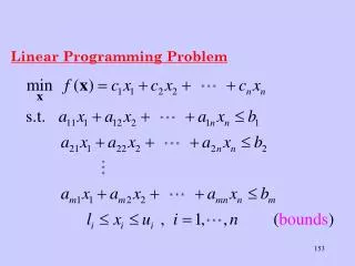
3. Linear Programming (LP) Problem • If both the objective and the constraints can be written as linear functions, the problem is referred to as a linear programming problem. • Linear functions are functions in which each variable appears in a separate term raised to the first power and is multiplied by a constant (which could be 0). • Linear constraints are linear functions that are restricted to be "less than or equal to", "equal to", or "greater than or equal to" a constant. • The objective value that you are attempting to minimize or maximize is referred to as the objective function. Dr. C. Lightner Fayetteville State University

4. Examples of Linear Functions Assume that x, y, and z are decision variables. Identify the valid linear functions below. • 5xy • x/y + 2z • 4x + 3y + (2/3)z • 5x2 + 6y2 • 2 + x • (x + y) / z Dr. C. Lightner Fayetteville State University

5. Linear Function Example Answer C and E are the only valid linear functions. These are the only functions with no more than one variable in a single term. Furthermore, the exponents on the variables are 0 or 1 (Recall that anything with a 0 exponent is 1. Thus 2*z0 equals 2*1=1, therefore the 2 in a single term satisfies the linear function requirements). Dr. C. Lightner Fayetteville State University

6. Problem Formulation Problem formulation or modeling is the process of translating a verbal statement of a problem into a mathematical statement. Dr. C. Lightner Fayetteville State University

7. Guidelines for Model Formulation • Understand the problem thoroughly. • Describe the objective in words. • Describe each constraint in words. • Define the decision variables. • Write the objective in terms of the decision variables. • Write the constraints in terms of the decision variables. Dr. C. Lightner Fayetteville State University

8. PAR, Inc Example Par, Inc manufactures golf equipment and supplies. The company wants to produce standard and deluxe golf bags. Par profits $10 for each Standard bag produced and sold, and $9 for each Deluxe bag produced and sold. Par’s distributor has agreed to purchase all golf bags that are produced by Par for the next three months. Par has the following operations for the production of bags 1. Cutting and dyeing the material 2. Sewing 3. Finishing (Inserting umbrella holder, club separators, etc.) 4. Inspection and packaging © 2003 Thomson/South-Western Dr. C. Lightner Fayetteville State University

9. Table of Production Requirements and Resources © 2003 Thomson/South-Western Dr. C. Lightner Fayetteville State University

10. Formulating Par, Inc Example OBJECTIVE: To maximize profits CONSTRAINTS: • # of hours dedicated to cutting and dyeing must be less than or equal to the number of available hours. • # of hours dedicated to sewing must be less than or equal to the number of available hours. • # of hours dedicated to finishing must be less than or equal to the number of available hours. • # of hours dedicated to inspecting and packaging must be less than or equal to the number of available hours. • All decision variables must be nonnegative. Don’t forget this one Dr. C. Lightner Fayetteville State University

11. Par Inc Problem Formulation (continued) DECISION VARIABLES: x1 - # of Standard bags to produce x2- # of Deluxe bags to produce In general, xj is the generic variable name for all decision variables. The variable, xj represents the jth decision variable. Dr. C. Lightner Fayetteville State University

12. Par Inc Problem Formulation (continued) • Using these decision variables our objective is to maximize profits. If we produce x1 Standard bags and x2 Deluxe bags our profits would be 10 x1 + 9 x2. Thus our objective function can be stated as Maximize 10 x1 + 9 x2 Dr. C. Lightner Fayetteville State University

13. Par Inc Problem Formulation (continued) • If we produce x1 Standard bags and x2 Deluxe bags, then we would utilize 7/10 x1 + 1 x2 hours of Cutting and Dyeing. We only have 630 hours available, thus we must ensure that 7/10 x1+ 1 x2 ≤ 630. • We would use 1/2 x1+ 5/6 x2 hours of Sewing. We must ensure that 1/2 x1+ 5/6 x2 ≤ 600. • We would use 1 x1+ 2/3 x2 hours of Finishing. We must ensure that 1 x1+ 2/3 x2 ≤ 708. • We would use 1/10 x1+ 1/4 x2 hours of Inspection and Packing. We must ensure that 1/10 x1+ 1/4 x2 ≤ 135. • We must make sure that a nonnegative number of bags are produced. Thus x1 ≥ 0 and x2 ≥ 0. Dr. C. Lightner Fayetteville State University

14. Par Inc LP model • Collectively our objective function and constraints can be written as the following linear programming model: Maximize 10 x1 + 9 x2 Subject to: 7/10 x1 + 1 x2 ≤ 630 1/2 x1 + 5/6 x2 ≤ 600 1 x1 + 2/3 x2 ≤ 708 1/10 x1+ 1/4 x2 ≤ 135 x1 ≥ 0 x2 ≥ 0 Dr. C. Lightner Fayetteville State University

15. Floataway Tours Example Floataway Tours has $420,000 that may be used to purchase new rental boats for hire during the summer. The boats can be purchased from two different manufacturers. Floataway Tours would like to purchase at least 50 boats and would like to purchase the same number from Sleekboat as from Racer to maintain goodwill. At the same time, Floataway Tours wishes to have a total seating capacity of at least 200. Pertinent data concerning the boats are summarized on the next slide. Formulate this problem as a linear program to maximize the daily expected profit. © 2003 Thomson/South-Western Dr. C. Lightner Fayetteville State University

16. Floataway Tours Example Data Maximum Expected Boat Builder Cost Seating Daily Profit Speedhawk Sleekboat $6000 3 $ 70 Silverbird Sleekboat $7000 5 $ 80 Catman Racer $5000 2 $ 50 Classy Racer $9000 6 $110 © 2003 Thomson/South-Western Dr. C. Lightner Fayetteville State University

17. Floataway Tours Example (continued) • Define the decision variables x1 = number of Speedhawks ordered x2 = number of Silverbirds ordered x3 = number of Catmans ordered x4 = number of Classys ordered • Define the objective function Maximize total expected daily profit or Max 70x1 + 80x2 + 50x3 + 110x4 Dr. C. Lightner Fayetteville State University

18. Floataway Tours Example (continued) • Define the constraints (1) Spend no more than $420,000: 6000x1 + 7000x2 + 5000x3 + 9000x4< 420,000 (2) Purchase at least 50 boats: x1 + x2 + x3 + x4> 50 (3) Number of boats from Sleekboat equals number of boats from Racer: x1 + x2 = x3 + x4 or x1 + x2 - x3 - x4 = 0 Constraints should always be written with all variables on one side and just a constant on the other. Dr. C. Lightner Fayetteville State University

19. Floataway Tours Example (continued) • Define the constraints (continued) (4) Capacity at least 200: 3x1 + 5x2 + 2x3 + 6x4> 200 Nonnegativity of variables: x1> 0 x2> 0 x3> 0 x4> 0 Dr. C. Lightner Fayetteville State University

20. Floataway Tours LP Formulation Max 70x1 + 80x2 + 50x3 + 110x4 s.t. 6000x1 + 7000x2 + 5000x3 + 9000x4< 420,000 x1 + x2 + x3 + x4> 50 x1 + x2 - x3 - x4 = 0 3x1 + 5x2 + 2x3 + 6x4> 200 x1> 0 x2 > 0 x3 > 0 x4> 0 Dr. C. Lightner Fayetteville State University

21. U.S. Navy Example The Navy produces up to 8,800 pounds of material in Albany, Georgia which it ships to three installations: San Diego, Norfolk, and Pensacola. They require at least 3,700, 2,500, and 2,500 pounds, respectively. In order to maintain outsourcing contracts, they must ship at least 2000 pounds via each mode of transportation (truck, railroad, and airplane). The shipping costs per pound for truck, railroad, and airplane transit are shown on the next slide. Formulate and solve a linear program to determine the shipping arrangements (mode, destination, and quantity) that will minimize the total shipping cost. © 2003 Thomson/South-Western Dr. C. Lightner Fayetteville State University

22. U.S. Navy Example Data Destination Mode San Diego Norfolk Pensacola Truck $12 $ 6 $ 5 Railroad 20 11 9 Airplane 30 26 28 © 2003 Thomson/South-Western Dr. C. Lightner Fayetteville State University

23. U.S. Navy Example Define the Decision Variables We want to determine the pounds of material, x ij , to be shipped by mode i to destination j. The following table summarizes the decision variables: San Diego Norfolk Pensacola Truckx11x12x13 Railroad x21x22x23 Airplane x31x32x33 © 2003 Thomson/South-Western Dr. C. Lightner Fayetteville State University

24. U.S. Navy Example (Continued) Define the Objective Function Minimize the total shipping cost. Min: (shipping cost per pound for each mode per destination pairing) x (number of pounds shipped by mode per destination pairing). Min 12x11 + 6x12 + 5x13 + 20x21 + 11x22 + 9x23 + 30x31 + 26x32 + 28x33 Dr. C. Lightner Fayetteville State University

25. U.S. Navy Example (Continued) Define the Constraints Destination material requirements: x11 + x21 + x31 ≥ 3700 (San Diego requirement) x12 + x22 + x32 ≥ 2500 (Norfolk requirement) x13 + x23 + x33 ≥ 2500 (Pensacola requirement) Maintain outsourcing contracts: x11 + x12 + x13 ≥ 2000 (Truck) x21 + x22 + x23 ≥ 2000 (Railroad) x31 + x32 + x33 ≥ 2000 (Airplane) Do not exceed 8800 pounds available x31 + x32 + x33+x11 + x12 + x13 + x21 + x22 + x23≤8800 Dr. C. Lightner Fayetteville State University

26. U.S. Navy Example (Continued) Nonnegativity of variables: x11> 0 x12> 0 x13> 0 x21> 0 x22> 0 x23> 0 x31> 0 x32> 0 x33> 0 Dr. C. Lightner Fayetteville State University

27. U.S. Navy LP Formulation Min 12x11 + 6x12 + 5x13 + 20x21 + 11x22 + 9x23 + 30x31 + 26x32 + 28x33 s.t. x11 + x21 + x31 ≥ 3700 x12 + x22 + x32 ≥ 2500 x13 + x23 + x33 ≥ 2500 x11 + x12 + x13 ≥ 2000 x21 + x22 + x23 ≥ 2000 x31 + x32 + x33 ≥ 2000 x31 + x32 + x33+x11 + x12 + x13 + x21 + x22 + x23≤8800 x11> 0, x12> 0, x13> 0, x21> 0, x22> 0, x23> 0, x31> 0, x32> 0, x33> 0 Dr. C. Lightner Fayetteville State University

28. Police Scheduling Problem The Clark County Sheriff’s department schedules police officers for 8-hour shifts. The beginning times for the shifts are 8:00AM, noon, 4:00PM, 8:00PM, midnight and 4AM. An officer beginning a shift at of these times works for the next 8 hours. During normal and weekday operations, the number of officers needed varies depending on the time of the day. The department staffing guidelines require the following minimum number of officers on duty. Time of Day Minimum officers on Duty 8:00AM – Noon 5 Noon – 4:00PM 6 4:00PM – 8:00PM 10 8:00PM – Midnight 7 Midnight – 4:00AM 4 4:00AM – 8:00AM 6 The Department wants to minimize the total number of officers needed to meet all shift requirements. Anderson, Sweeney, and Williams Dr. C. Lightner Fayetteville State University

29. Police Scheduling Problem Develop a linear program for this problem that will determine the number of officers that should be scheduled to begin the 8-hour shifts at each of the six times (8:00AM, noon, 4:00PM, 8:00PM, midnight and 4AM) in order to minimize the total number of officers required. (Hint: Let x1= the number of officers beginning work at 8AM, x2 = the number of officers beginning work at noon and so on.) Dr. C. Lightner Fayetteville State University

30. Police Scheduling Problem (Continued) Define Variables x1= # of officers that begin work at 8AM & work shifts (8AM - Noon) & (Noon to 4PM) x2= # of officers that begin work at Noon & work shifts (Noon - 4PM) & (4PM - 8PM) x3= # of officers that begin work at 4PM & work shifts (4PM – 8PM) & (8PM to Midnight) x4= # of officers that begin work at 8PM & work shifts (8PM - Midnight) & (Midnight – 4AM) x5= # of officers that begin work at Midnight & work shifts (Midnight – 4AM) & (4AM to 8AM) x6= # of officers that begin work at 4AM & work shifts (4AM – 8AM) & (8AM - Noon) Dr. C. Lightner Fayetteville State University

31. Police Scheduling Problem (Continued) Define the Objective Function Minimize the total number of officers needed to meet all shift requirements. Or Min x1 + x2 + x3 + x4 + x5 + x6 Dr. C. Lightner Fayetteville State University

32. Police Scheduling Problem (Continued) Define the Constraints Each shift must have at least the minimum number of officers • x6+x1 ≥ 5 • x1+x2 ≥ 6 • x2+x3 ≥ 10 • x3+x4 ≥ 7 • x4+x5 ≥ 4 • x5+x6 ≥ 6 Nonnegativity constraints x1≥ 0, x2≥ 0,x3≥ 0, x4 ≥ 0, x5 ≥ 0, x6≥ 0 Dr. C. Lightner Fayetteville State University

33. Police Scheduling LP Formulation Min x1 + x2 + x3 + x4 + x5 + x6 s.t. x6+x1 ≥ 5 x1+x2 ≥ 6 x2+x3 ≥ 10 x3+x4 ≥ 7 x4+x5 ≥ 4 x5+x6 ≥ 6 x1≥ 0, x2≥ 0,x3≥ 0, x4 ≥ 0, x5 ≥ 0, x6≥ 0 Dr. C. Lightner Fayetteville State University

34. THE END See your textbook for more examples and detailed explanations of all topics discussed in these notes. Dr. C. Lightner Fayetteville State University