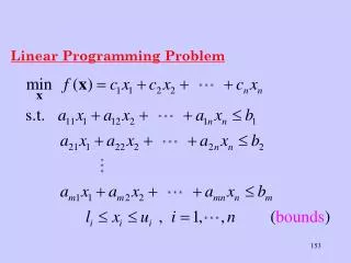
Linear Programming Problem
Learn about the simplex algorithm, genetic algorithms, and optimal solutions for linear programming problems. Explore MATLAB optimization tools and the application of genetic algorithms in search and optimization.

Linear Programming Problem
E N D
Presentation Transcript
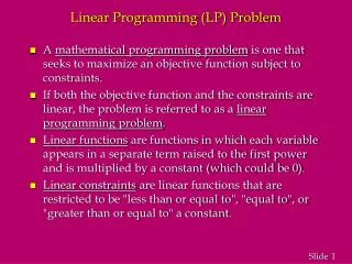
which can be written in the form:- Assuming a feasible solution exists it will occur at a corner of the feasible region. That is at an intersection of equality constraints. The simplex linear programming algorithm systematically searches the corners of the feasible region in order to locate the optimum.
Consider the problem: Example:
Plotting contours of f(x) and the constraints produces: 4 x 10 3 f increasing 2.5 2 1.5 x 2 1 0.5 0 0 0.5 1 1.5 2 2.5 3 3.5 4 x 4 x 10 1 (a) (c) solution (b)
The maximum occurs at the intersection of (a) and (b):- intersection x f x =0, (c) (0, 16,667) 180,000 1 (b), (c) (15,000, 12,500) 256,500 (a), (b) (26,207, 6,897) 286,760 max (a), x =0 (30,000, 0) 243,000 2 At the other intersections (corners) of the feasible region:
DEMO Solution using MATLAB Optimisation Toolbox Routine LP
GENETIC ALGORITHMS Refs: - Goldberg, D.E.: ‘ Genetic Algorithms in Search, Optimization and Machine Learning’ (Addison Wesley,1989) Michalewicz, Z.: ‘Genetic Algorithms + Data Structures = Evolution Programs’ (Springer Verlag, 1992)
Genetic Algorithmsare search algorithms based on the mechanics of natural selectionand natural genetics. They start with a group of knowledge structures which are usually coded into binary strings (chromosomes). These structures are evaluated within some environment and the strength (fitness) of a structure is defined. The fitness of each chromosome is calculated and a new set of chromosomes is then formulated by random selection and reproduction. Each chromosome is selected with a probability determined by it’s fitness and, hence, chromosomes with the higher fitness values will tend to survive and those with lower fitness values will tend to become extinct.
“Survival of the fittest” The selected chromosomes then undergo certain genetic operations such as crossover, where chromosomes are paired and randomly exchange information, and mutation, where individual chromosomes are altered. The resulting chromosomes are re-evaluated and the process is repeated until no further improvement in overall fitness is achieved. In addition, there is often a mechanism to preserve the current best chromosome (elitism).
Initial Population and Coding Selection “survival of the fittest” Elitism Crossover Mating Mutation Genetic Algorithm Flow Diagram
Components of a Genetic Algorithm (GA) • a genetic representation • a way to create an initial population of potential solutions • an evaluation function rating solutions in terms of their “fitness” • genetic operatorsthat alter the composition of children during reproduction • values of various parameters (population size, probabilities of applying genetic operators, etc)
Differences from Conventional Optimisation • GAs work with a coding of the parameter set, not the parameters themselves • GAs search from a population of points, not a single point • GAs use probabilistic transition rules, not deterministic rules • GAs have the capability of finding a global optimumwithin a set of local optima
Consider the problem: where, without loss of generality, we assume that f is always +ve (achieved by adding a +ve constant if necessary). Also assume: Suppose we wish to represent xi to d decimal places. That is each range needs to be cut into (bi-ai).10d equal sizes. Let mi be the smallest integer such that Then xi can be coded as a binary string of length mi. Also, to interpret the string, we use: Initial Population and Coding
Each chromosome (population member) is represented by a binary string of length: where the first m1 bits map x1 into a value from the range [a1,b1], the next group of m2 bits map x2 into a value from the range [a2,b2] etc; the last mn bits map xn into a value from the range [an,bn]. To initialise a population, we need to decide upon the number of chromosomes (pop_size). We then initialise the bit patterns, often randomly, to provide an initial set of potential solutions.
Selection (roulette wheel principle) We mathematically construct a ‘roulette wheel’ with slots sized according to fitness values. Spinning this wheel will then select a new population according to these fitness values with the chromosomes with the highest fitness having the greatest chance of selection. The procedure is:
1) Calculate the fitness value eval(vi) for each chromosome vi (i = 1,...,pop_size) 2) Find the total fitness of the population 3) Calculate the probability of a selection, pi, for each chromosome vi (i = 1,...,pop_size) 4) Calculate a cumulative probability qi for each chromosome vi (i = 1,...,pop_size)
The selection process is based on spinning the roulette wheel pop_size times; each time we select a single chromosome for a new population as follows: 2) If r < q1, select the first chromosome v1; otherwise select the ith chromosome vi such that: 1) Generate a random number r in the range [0,1] Note that some chromosomes would be selected more than once: the best chromosomes get more copies and worst die off. “survival of the fittest” All the chromosomes selected then replace the previous set to obtain a new population.
example: p10 p11 p12 p9 p1 p8 p2 p7 p3 p6 p5 p4 segment area proportional to pi, i=1,...,12
Crossover We choose a parameter value pc as the probability of crossover. Then the expected number of chromosomes to undergo the crossover operation will be pc.pop_size. We proceed as follows:- (for each chromosome in the new population) 1) Generate a random number r from the range [0,1]. 2) If r < pc, then select the given chromosome for crossover. ensuring that an even number is selected. Now we mate the selected chromosomes randomly:-
For each pair of chromosomes we generate a random number pos from the range [1,m-1], where m is the number of bits in each chromosome. The number pos indicates the position of the crossing point. Two chromosomes: are replaced by a pair of their offspring (children)
Mutation We choose a parameter value pm as the probability of mutation. Mutation is performed on a bit-by-bit basis giving the expected number of mutated bits as pm.m.pop_size. Every bit, in all chromosomes in the whole population, has an equal chance to undergo mutation, that is change from a 0 to 1 or vice versa. The procedure is: For each chromosome in the current population, and for each bit within the chromosome:- 1) Generate a random number r from the range [0,1]. 2) If r < pm, mutate the bit.
Elitism It is usual to have a means for ensuring that the best value in a population is not lost in the selection process. One way is to store the best value before selection and, after selection, replace the poorest value with this stored best value.
3 global max 2.5 2 1.5 f(x) 1 0.5 0 -0.5 -1 -1 -0.5 0 0.5 1 1.5 2 x Example
Let us work to a precision of two decimal places. then the chromosome length m must satisfy: Also let pop_size = 10, pc = 0.25, pm = 0.04 To ensure that a positive fitness value is always achieved we will work on val = f(x) + 2
Note for v1: Consider that the initial population has been randomly selected as follows (giving also the corresponding values of x, val, probabilities and accumulated probabilities) * fittest member of the population
Selection Assume 10 random numbers, range [0,1], have been obtained as follows:- 0.47 0.61 0.72 0.03 0.18 0.69 0.83 0.68 0.54 0.83 These will select: 0.47 0.61 0.72 0.03 0.18 0.69 0.83 0.68 0.54 0.83 v4 v6 v8 v1 v2 v7 v9 v7 v5 v9 giving the new population:
Note that the best chromosome v3 in the original population has not been selected and would be destroyed unless elitism is applied.
Crossover (pc = 0.25) Assume the 10 random numbers:- 12345678910 0.07 0.94 0.57 0.36 0.31 0.14 0.60 0.070.07 1.00 These will select v1, v6, v8, v9 for crossover. Now assume 2 more random numbers in the range [1,8] are obtained:-
no change produces Mating v1 and v6 crossing over at bit 8:- Mating v8 and v9 crossing over at bit 4:- giving the new population:-
mutation (pm = 0.04) Suppose a random number generator selects bit 2 of v2 and bit 8 of v9 to mutate, resulting in:- ** weakest Total fitness F = 30.54
Elitism So far the iteration has resulted in a decrease in overall fitness (from 32.08 to 30.54). However, if we now apply elitism we replace v8 in the current population by v3 from the original population, to produce: Total fitness F = 32.61
resulting now in an increase of overall fitness (from 32.08 to 32.61) at the end of the iteration. The GA would now start again by computing a new roulette wheel and repeating selection, crossover, mutation and elitism; repeating this procedure for a pre-selected number of iterations.
Final results from a MATLAB GA program using parameters: pop_size = 30, m = 22, pc = 0.25, pm=0.01
Tabulated results: x val x val x val 1.8500 4.8500 1.8503 4.8502 1.8500 4.8500 1.8496 4.8495 1.8500 4.8500 1.8500 4.8500 0.3503 2.6497 1.8504 4.8502 1.8269 4.3663 1.8504 4.8502 1.8503 4.8502 1.8500 4.8500 1.8265 4.3520 1.8503 4.8502 1.8386 4.7222 1.8500 4.8500 1.8496 4.8495 1.8500 4.8500 1.8503 4.8502 1.8504 4.8502 1.8500 4.8500 1.8500 4.8500 1.8503 4.8502 1.8500 4.8500 1.8496 4.8495 1.8496 4.8495 1.8503 4.8502 1.8500 4.8500 1.8500 4.8500 1.8968 3.1880 The optimum val = 4.8502 at x = 1.8504 Hence: remembering that val(x) = f(x) + 2
ON-LINE OPTIMISATION - INTEGRATED SYSTEM OPTIMISATION AND PARAMETER ESTIMATION (ISOPE) An important application of numerical optimisation is the determination and maintenance of optimal steady-state operation of industrial processes, achieved through selection of regulatory controller set-point values. Often, the optimisation criterion is chosen in terms of maximising profit, minimising costs, achieving a desired quality of product, minimising energy usage etc. The scheme is of a two-layer hierarchical structure:-
OPTIMISATION (based on steady-state model) set points REGULATORY CONTROL e.g. PID Controllers control signals measurements INDUSTRIAL PROCESS inputs outputs Note that the steady-state values of the outputs are determined by the controller set-points assuming, of course, that the regulatory controllers maintain stability.
The set points are calculated by solving an optimisation problem, usually based on the optimisation of a performance criterion (index) subject to a steady-state mathematical model of the industrial process. Note that it is not practical to adjust the set points directly using a ‘trial and error’ technique because of process uncertainty and non-repeatability of measurements of the outputs. Inevitably, the steady-state model will be an approximation of the real industrial process, the approximation being both in structure and parameters. We call this the model-reality difference problem.
ROP - Real Optimisation Problem • Complex • Intractable • MOP - Model Based Optimisation Problem • Simplified (e.g... Linear - Quadratic) • Tractable ??? Can We Find the Correct Solution of ROP By Iterating on MOP in an Appropriate Way YES By Applying Integrated System Optimisation And Parameter Estimation - ISOPE ISOPE Principle
Iterative Optimisation and Parameter Estimation In order to cope with model-reality differences, parameter estimation can be used giving the following standard two-step approach:-
1. Apply current set points values and, once transients have died away, take measurements of the real process outputs. use these measurements to estimate the steady-state model parameters corresponding to these set point values. This is the parameter estimation step. 2. Solve the optimisation problem of determining the extremum of the performance index subject to the steady-state model with current parameter values. This is the optimisation stepand the solution will provide new values of the controller set points. The method is iterative applied through repeated application of steps 1 and 2 until convergence is achieved.
y PARAMETER ESTIMATION MODEL BASED OPTIMISATION y* c REGULATORY CONTROL y* REAL PROCESS Standard Two-Step Approach
Example real solution Now consider the two-step approach:- parameter estimation
optimisation i.e. This first-order difference equation will converge (i.e. stable) since and Hence, at iteration k:
HENCE, THE STANDARD TWO STEP APPROACH DOES NOT CONVERGE TO THE CORRECT SOLUTION!!! final solution
Integrated Approach The standard two-step approach fails, in general, to converge to the correct solution because it does not properly take account of the interaction between the parameter estimation problem and the system optimisation problem. Initially, we use an equality v = c to decouple the set points used in the estimation problem from those in the optimisation problem. We then consider an equivalent integrated problem:-
This is clearly equivalent to the real optimisation problem ROP
If we also write the model based optimisation problem as: (by eliminating y in J(c,y)) giving the equivalent problem:-
Form the Lagrangian: with associated optimality conditions: together with:-