Unlocking Efficiency with Linear Programming
Discover how linear programming optimizes real-world scenarios such as crew scheduling, production planning, and network design. Learn about applications in airline operations, minimizing excess cost in crew pairing, and fleet assignment in the airline industry. Explore solving linear equations, maximizing flow, and finding optimal solutions in a minimum spanning tree. Embrace the power of linear programming in decision-making for cost-effective solutions.

Unlocking Efficiency with Linear Programming
E N D
Presentation Transcript
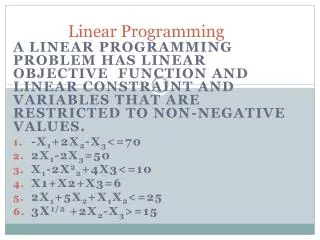
Linear Programming • The process of minimizing a linear objective function subject to a finite number of linear equality and inequality constraints. • Example applications: • airline crew scheduling • manufacturing and production planning • portfolio selection • telecommunications network design • “Few problems studied in computer science have greater application in the real world.”
Network flow is a linear programming problem • - flow function is the set of unknowns • - conservation is a set of linear equations • - capacity constraints are linear inequalities • - maximum flow requirement is a linear objective function to be maximized. • What about minimum spanning tree problem? • - Each edge has a weight 1 (chosen) 0 (else). • - constraint of acyclicity: for each cycle C, if edges in it are e1, e2, …, ek, then • x1 + x2 + … + xk <= k-1 would do it.
- connectedness: x1 + x2 + … + xe = v – 1 Objective function: w1 x1 + w2 x2 + … + we xe Although this is not the right way to solve MST problem, this argument shows that it is a special case of linear programming problem. Maximum matching in a bipartite graph: How can it be expressed as a linear programming problem?
Big Bucks! “American Airlines employs more than 25,000 pilots and flight attendants to fly its fleet of over 600 aircraft. Crew cost is over 1.3 billion dollars per year is second only to fuel cost. In its effort to better utilize crew resources AA spent about 6000 hours of CPU time during 1989-90 running its crew-pairing code… Estimated savings generated by running this code during the past 5 years are in excess of 20 million dollars per year. A crew pairing is a sequence of flights that starts and ends at a crew base and typically lasts 2-3 days. A crew member works 4-5 pairings per month. The most important part of efficient crew utilization is making up pairings that cover all flight legs and minimize excess cost. This problem is called crew-pairing optimization.”
And more... Delta Air Lines flies over 2,500 domestic flight legs every day, using about 450 aircraft from 10 different fleets. The fleet assignment problem is to match aircraft to flight legs so that seats are filled with paying passengers. Recent advances in mathematical programming algorithms and computer hardware make it possible to solve optimization problems of this scope for the first time. Delta is the first airline to solve to completion one of the largest and most difficult problems in this industry. Use of the Coldstart model is expected to save Delta Air Lines $300 million over the next three years.
Linear equations A x = b where A is a n by n matrix, b is a n x 1 column vector, x is a column of variables. - if A-1 exists, then the system has a unique solution, x = A-1 b. - time taken to solve a system of equations is typically O(n3) where n is the number of variables. - note that this bound is O(n1.5) in terms of the problem size.
But when linear inequalities are involved, the number of solutions is typically infinite. Example: x + 2 y <= 12, 3x + y <= 31
Feasible Set • Each linear inequality divides n-dimensional space into two half-spaces, one where the inequality is satisfied, and one where it’s not. • Feasible Set : solutions to a family of linear inequalities. • Family of linear cost functions, gives family of parallel hyper-planes (lines in 2D, planes in 3D, etc.). Want to find one of minimum cost => must occur at corner of feasible set.
An example: The diet problem • Trying to decide on lowest cost diet that provides sufficient amount of protein, with two choices: • steak: 2 units of protein/pound, $3/pound • peanut butter: 1 unit of protein/pound, $2/pound • In proper diet, need 4 units protein/day. Goal: minimize 2x + 3y subject to constraints: x + 2y >= 4 x = # pounds peanut butter/day in optimal diet >=0 y = # pounds steak/day in optimal diet >=0
y=0 feasible set x=0 x+2y=4 Visually…x= peanut butter, y = steak
Optimal vector occurs at corner of feasible set! y=0 feasible set x=0 x+2y=4 2x+3y=6 2x+3y=0
Optimal vector occurs at corner of feasible set! y=0 feasible set x=0
General Form of a Linear Program Minimize b1y1 + b2y2 +…+ bmym subject to S1<=i<= m aijyi >= cj j=1..n yi >= 0 i=1..m or Maximize c1x1 + c2x2 +…+ cnxn subject to S1<=j<= n aijxj <= bj i=1..m xj>= 0 j=1..n
The Feasible Set • Intersection of a set of half-spaces, called a polyhedron. • If it’s bounded and nonempty, it’s a polytope 3 cases: - feasible set is empty • - cost function is unbounded on feasible set. • - cost has a minimum (or maximum) on feasible set. First two cases very uncommon for genuine problems in economics and engineering.
The Simplex Method • Phase I : locate a corner of the feasible set. • corner = intersection of n different planes (in n dimensions) • Phase II: move from corner to corner along the edges of the feasible set -- always go along an edge that is guaranteed to decrease the cost. • Edge = intersection of n-1 different planes • When reach a local minimum (maximum), you’ve found the optimum.
Simplex Algorithm: An Example in 3D Maximize 5x + 4y + 3z subject to 2x+ 3y + z <= 5 4x + y + 2z <= 11 3x + 4y + 2z <= 8 x,y,z >=0. Step 0:convert inequalities into equalities by introducing slack variables a,b,c. Define: a = 5-2x-3y-z => a >=0 b = 11-4x-y-2z => b >=0 c = 8-3x-4y-2z => c >=0 F = 5x+4y + 3z, objective function
Example of Simplex Method, continued. Step 1: Find initial feasible solution: x=0, y=0, z=0 => a=5, b=11, c=8 => F=0. Step 2: Find feasible solution with higher value of F For example, can increase x to get F=5x. How much can we increase x? a = 5-2x-3y-z >=0 => x <= 5/2 most stringent b = 11-4x-y-2z >=0 => x <= 11/4 c = 8-3x-4y-2z >=0 => x <= 8/3 => increase x to 5/2 =>F= 25/2, a=0, b=1, c=1/2
Example of Simplex Method, continued. Want to keep doing this, need to get back into state where x,b,c on l.h.s. of equations. a = 5-2x-3y-z => x= 5/2 -3/2 y -1/2 z - 1/2 a (*) Substituting (*) into other equations: b = 11-4x-y-2z >=0 => b = 1 + 5y + 2a c = 8-3x-4y-2z >=0 => c = 1/2 + 1/2 y -1/2 z + 3/2 a F = 5x+4y + 3z => F= 25/2 - 7/2 y + 1/2 z - 5/2 a In order to increase F again, should increase
Example of Simplex Method, continued. How much can we increase z? x= 5/2 -3/2 y -1/2 z - 1/2 a => z <= 5 b = 1 + 5y + 2a => no restriction c = 1/2 + 1/2 y -1/2 z + 3/2 a => z <= 1 most stringent (^) Setting z = 1 yields x=2, y=0, z=1, a=0, b = 1, c = 0. F= 25/2 - 7/2 y + 1/2 z - 5/2 a => F= 13. Again, construct system of equations. From (^) z = 1 + y + 3a - 2c.
Example of Simplex Method, continued. Substituting back into other equations: z = 1 + y + 3a - 2c. x= 5/2 -3/2 y -1/2 z - 1/2 a => x = 2-2y-2a + c b = 1 + 5y + 2a => b= 1 + 5y + 2a F = 25/2 - 7/2 y + 1/2 z - 5/2 a => F = 13 - 3y -a - c And we’re done.
The Simplex Method • Phase I : locate a corner of the feasible set. • corner = intersection of n different planes (in n dimensions) • Phase II: move from corner to corner along the edges of the feasible set -- always go along an edge that is guaranteed to decrease the cost. • Edge = intersection of n-1 different planes • When reach a local minimum (maximum), you’ve found the optimum.
What were we doing? • Each time we had a feasible solution we were at a corner == a meeting point of 3 different planes. We chose 3 variables and set them to 0, and made sure remaining constraints were satisfied. • Then we moved along an edge == a meeting point of 2 different planes obtained from corner by removing one equation. Moved along associated edge until arrived at a new corner.
The Simplex Algorithm and beyond…. • In practice, quite fast -- typically only O(m) pivots (where m is the number of constraints) • In worst case, exponential. • For a long time, it wasn’t known if there was a polynomial time algorithm until…. • Khachian’s algorithm “The Mathematical Sputnik of 1979” • exterior-point method • And then there was Karmakar (1984)… • interior-point method • competes viably with simplex algorithm on real-world problems.
A Central Result of LP TheoryDuality Theorem • Every linear program has a dual • If the original is a minimization, the dual is a maximization and vice versa • Solution of one leads to solution of other Primal: Minimize cx subject to Ax >= b, x>=0 Dual: Maximize yb subject to yA <=c, y>=0 If one has optimal solution so does other, and their values are the same.
Primal: Minimize cx subject to Ax >= b, x>=0Dual: Maximize yb subject to yA <=c, y>=0 • In the primal, c in cost function and b was in the constraint. In the dual, reversed. • Inequality sign is changed and minimization turns to maximization. • Example: minimize 2x + 3y subject to x+2y>=4, 2x + 5y >= 1, x - 3y >= 2, x>=0, y>=0 • Dual problem: maximize 4p +q + 2r subject to p+2q + r <= 2, 2p+5q -3r <= 3, p,q,r >=0
An example: The diet problem • Trying to decide on lowest cost diet that provides sufficient amount of protein, with two choices: • steak: 2 units of protein/pound, $3/pound • peanut butter: 1 unit of protein/pound, $2/pound • In proper diet, need 4 units protein/day. Goal: minimize 2x + 3y subject to constraints: x + 2y >= 4 x = # pounds peanut butter/day in optimal diet >=0 y = # pounds steak/day in optimal diet >=0
Simple Example • Diet problem: minimize 2x + 3y subject to x+2y>=4, x>=0, y>=0 • Dual problem: maximize 4p subject to p<=2, 2p <=3, p>=0 • Dual: the problem faced by a druggist who sells synthetic protein, trying to compete with peanut butter and steak • He wants to maximize the price p, subject to constraints: • synthetic protein must not cost more than protein • price must be non-negative or he won’t sell any • revenue to druggist will be 4p • Solution: p<= 3/2 => objective function = 4p = 6 • Not coincidence that it’s = minimal cost in original problem.
More general diet problem Minimum problem has n unknowns, n foods to be eaten in amounts x1,… , xn m constraints represent m required vitamins • entry aijis amount of i-th vitamin in j-th food. • i-th row of Ax >=b forces the diet to include that vitamin in at least the amount bi. • c1x1 + …. + cnxn = cost of diet (cj is cost of j-th food.) Dual -- druggist selling vitamin pills rather than food. • Prices adjustable as long as nonnegative. • Key constraint -- on each food can’t charge more than grocer. • Since food j contains vitamins in amount aij , the druggist’s price for the equivalent in vitamins can’t exceed cj => yA <= c. • Can then sell amount bi of each vitamin for a total income of y1b1+..+ ymbm
Example Minimize c(st) x(st) + c(pb) x(pb) subject to • prot(st) x(st) + prot(pb) x(pb) >= q(prot) • carbo(st) x(st) + carbo(pb) x(pb) >= q(carbo) • x(st), x(pb) >= 0 • c(n) = per unit cost of food n, x(n) quantity of food n to purchase per day, prot(n) = units protein per unit of food n, carbo (n) = units carbo per unit n q(prot) = protein units per day needed, q(carbo) = carbo units per day Dual -- druggist selling synthetic protein and carbohydrate pills maximize q(prot) y(s-prot) + q(carbo) y(s-carbo) subject to • y(s-prot) prot(st) + y(s-carbo) carbo(st) <= c(st) • y(s-prot) prot(pb) + y(s-carbo) carbo(pb) <= c(pb) • y(s-prot), y(s-carbo) >= 0 • Can then sell amount q(prot) of protein per day and q(carbo) of carbo per day.
What’s going on? • Notice: feasible sets completely different for primal and dual, but nonetheless an important relation between them. • Duality theorem says that in the competition between the grocer and the druggist the result is always a tie. • Optimal solution to primal tells purchaser what to do. • Optimal solution to dual fixes the natural prices at which economy should run. • The diet x and vitamin prices y are optimal when • grocer sells zero of any food that is priced above its vitamin equivalent. • druggist charges 0 for any vitamin that is oversupplied in the diet.
Duality Theorem • Druggist’s max revenue = Purchasers min cost One direction of duality easy , for any feasible x, y: q(prot) y(s-prot) + q(carbo) y(s-carbo) <= x(st) c(st) + x(pb) c(pb) Since each food can be replaced by its vitamin equivalent, with no increase in cost, all adequate diets must be at least as expensive as any price the druggist would charge.
For [x(st), x(pb)] and [y(s-prot), y(s-carbo)] feasible => [prot(st) x(st) + prot(pb) x(pb)] y(s-prot) >= q(prot) y(s-prot) [carbo(st) x(st) + carbo(pb) x(pb)] y(s-carb) >= q(carbo) y(s-carb) Sum two inequalities => q(prot) y(s-prot) + q(carbo) y(s-carbo) <= [prot(st) x(st) + prot(pb) x(pb)] y(s-prot) + [carbo(st) x(st) + carbo(pb) x(pb)] y(s-carbo) = x(st) [y(s-prot) prot(st) + y(s-carbo) carbo(st) ] + x(pb) [y(s-prot) prot(pb) + y(s-carbo) carbo(pb)] <= x(st) c(st) + x(pb) c(pb) When they are equal, they both must be optimal.
Practical Use of Duality • Sometimes simplex algorithm (or other algorithms) will run faster on the dual than on the primal. • Can be used to bound how far you are from optimal solution. • Important implications for economists.
Formulate as LP • Want to invest $1000 in 3 stocks, <= $400 per • price/share dividends/year • stock A $50 $2 • stock B $200 $5 • stock C $20 0 • stock C has prob 1/2 of appreciating to $25 in a year, or (prob 1/2) staying same. • What amount of each stock should be bought to maximize dividends + expected appreciation over a year?
Application:Optimal Pipeline • A piece of data of size D goes through a pipeline of n stages. • Each stage has associated • oi -- overhead of i-th stage • bi -- bandwidth of i-th stage (bits/sec) • How should data be broken up into k pieces, not necessarily of equal size, so as to minimize time through the pipeline?
Summary of Linear Programming • Of great practical importance to solve linear programs: • they model important practical problems • production, approximating the solution of inconsistent equations, manufacturing, network design, flow control, resource allocation. • solving an LP is often an important component of solving or approximating the solution to an integer linear programming problem. • The simplex algorithm works very well in practice. • One problem where you really do not want to roll your own code.

