Linear Programming
Linear Programming. Reading: Chapter 4 of the Textbook Driving Applications Casting/Metal Molding Collision Detection Randomized Algorithms Smallest Enclosing Discs. Casting. Liquid metal is poured into a mold, it solidifies, and then the object shape is formed and the object is removed.

Linear Programming
E N D
Presentation Transcript
Linear Programming • Reading: Chapter 4 of the Textbook • Driving Applications • Casting/Metal Molding • Collision Detection • Randomized Algorithms • Smallest Enclosing Discs M. C. Lin
Casting • Liquid metal is poured into a mold, it solidifies, and then the object shape is formed and the object is removed. • Not all objects of different shapes can be removed. • Problems: Whether an object can be manufactured by casting; if so, find the suitable mold. M. C. Lin
Transform to a Geometric Problem • The shape of cavity in the mold is determined by the shape of the object, but different orientation can be crucial. • The object must have a horizontal top facet • Let P, object to be casted, be a 3D polyhedron bounded by planar facets with a designated top facet. Assume: the mold is rectangular block with a cavity that corresponds exactly to P. • Problem: Decide whether a direction d exists s.t. P can be translated to infinity in direction dwithout intersecting interior of of the mold. M. C. Lin
Problem Analysis • The polyhedron P can be removed from its mold by a translation in direction d if and only if d makes an angle of at least 90° with the outward normal of all ordinary facets of P. • Let n = (nx , ny , nz) be the outward normal of an ordinary facet. The direction d = (dx , dy , 1) makes an angle at least 90° with n if and only if the dot product of n and dis non-positive: nx dx + ny dy + nz 0 M. C. Lin
Problem Analysis (cont.) nx dx + ny dy + nz 0 • This describes a half-plane on the plane z=1, i.e. the area to the left or right of a line on the plane. • Casting problem: given a set of half-planes, find a point in their common intersection or decide if the common intersection is empty. • Let P be a polyhedron with n facets. In O(n2) expected time and using O(n) storage it can be decided whether P is castable. Moreover, if P is castable, a mold and a valid direction for removing P from it can be computed in the same amount of time. M. C. Lin
Half-Plane Intersection • Let H = {h1, h2, …, hn} be a set of linear constraints in two variables, i.e. in the form: ai x + bi y ci where ai , biand ci are constants, s.t. at least one of aiand bi is non-zero. • Problem: Find the set of all points (x,y) R2 that satisfy all n constraints at the same time; i.e. find all the points lying in the common intersection of the half-planes in H. M. C. Lin
Type of Intersections • Convex regions bounded by at most n edges (half-planes / lines) • Unbounded regions • Degenerate cases: a line or point • Empty M. C. Lin
IntersectHalfPlanes(H) Input: A set H of n half-planes in the plane Output: A convex polygonal region C:= hH h 1. if card(H) = 1 2. then C the unique half-plane h H 3. else Split H into sets H1and H2 of the size (n/2) and (n/2) 4. C1 IntersectHalfPlanes (H1) 5. C2 IntersectHalfPlanes (H2) 6. C IntersectConvexRegions(C1, C2) M. C. Lin
Run Time Analysis • Computing intersections of two overlays takes O( (n+k) log n) time, where k is the number of intersection points between edges of C1and edges of C2 and k n • T(n) = O(1), if n = 1 • T(n) = O(n log n) + 2 T(n/2), if n > 1 T(n) = O(n log2 n) M. C. Lin
Plane-Sweep for Half-Plane Intersection • Store left/right boundary of C as sorted lists of half-planes, Lleft(C) & Lright(C), in order from top to bottom. • Plane-Sweep: maintain edges of C1 & C2 intersecting the sweep line. There are at most four. Use pointers: l_edge_C1, r_edge_C1, l_edge_C2, r_edge_C2. • Initialization: (y1, y2) = y-coordinate of topmost of (C1 ,C2). If y1 has upward unbounded edge, y1 = . ystart=min(y1, y2) Initialize the pointers as ones intersecting ystart. M. C. Lin
Plane-Sweep for Half-Plane Intersection • Next event to be handled is the highest of the lower end points intersecting the sweep line. Use the pointers to find event points in constant time. • At each event point, some new edge e appears on the boundary. To handle edge e, we first check whether e belongs to C1 or C2, and whether it is on the left or right boundary, and then call appropriate procedure. • According to the handling of each case, we add the appropriate half-planes to the intersection of C1 & C2. All cases can be decided in constant time. M. C. Lin
Algorithm Analysis • It takes constant time to handle an edge. So, the intersection of two convex polygonal regions in the plane can be computed in O(n) time. So, now …... T(n) = O(n) + 2 T(n/2), if n > 1 T(n) = O(n logn) • The common intersection of a set of n half-planes in the plane can be computed in O(nlogn) time and linear storage. M. C. Lin
Linear Programming • Linear Programming/Optimization: finding a solution to a set of linear constraints Maximize c1 x1 + c2 x2 + … + cd xd ci Subject to a11 x1 + a12 x2 + … + a1d xd b1 a21 x1 + a22 x2 + … + a2d xd b2 : : an1 x1 + an2 x2 + … + and xd bn where aij , bi andci are real numbers and inputs M. C. Lin
LP Terminology • Objective Function: the funct. to be maximized • Linear Program: the objective functions and the set of constraints together • Dimension: the number of variables, d • Feasible Regions: the set of points satisfying all constraints. Points (solns) in this region are called “feasible” & points outside “infeasible”. M. C. Lin
2D Linear Programming • Let H be a set of nlinear constraints • The vector defining the obj. func. is c = (cx, cy) • The objective function is fc(p) = cx px + cy py • Problem: find a point p R2 s.t. p H and fc(p) is maximized. Denote the LP by (H, c) and its feasible region by C. M. C. Lin
Types of Solutions to 2D-LP 1. LP is infeasible, i.e. no solution 2. The feasible region is unbounded in direction c. There is a ray p completely contained in feasible region C, s.t. fc takes arbitrary large value along p 3. The feasible region has an edge e whose outward normal points in the direction c. The solution to LP is not unique: any point on e 4. There is a unique solution: a vertex v of C that is extreme in the directionc M. C. Lin
Optimal Vertex • In the case where an edge is a soln, there is an unique solution: lexicographically smallest one. • With this convention, we define “optimal vertex” as a vertex of the feasible region Based on this, we can incrementally add one constraint at a time and maintain the optimal vertex of the intermediate feasible regions, except in the case of unbounded LP. M. C. Lin
Incremental LP • If LP is unbounded, UnboundedLP() returns a ray. • If the LP is not unbounded, then UnboundedLP() returns 2 half-planes, h1 and h2 from H, s.t. ({h1 , h2}, c) is bounded. These half-planes are called certificates that proves (H, c)is really bounded. • Let Ci be the feasible region when the first i half-planes have been added: Ci:= h1 h2 … hi • Denote the optimal vertex of Ci by vi, clearly we have: C2 C3 C4 … Cn = C • If Ci= 0 for some i, then Cj= 0 for j i & LP infeasible M. C. Lin
How Optimal Vertex Changes • Let 2 < i n, let Ci and vi be defined as above. • If vi-1 hi , then vi = vi-1 • If vi-1 hi , then either Ci= 0 or vi li where liis the line bounding hi • Assume that the current optimal point vi-1 is not contained hi Restate the problem as: Find the point p on li that maximizes fc(p), subject to the constraints p hj, for 1 j i • Assume li is the x-axis. Let xjdenote x-coord. of the intersection point of li and lj. Depending on whether li is bounded to left/right, we geta constraint on the x-coord. of the solution of the form xxj or xxj M. C. Lin
Simplifying to 1D-LP Maximize fc((x,0)) Subject to x xj , 1 j< i and li hj bounded to left x xk , 1 k< i and lihk bounded to right • This is a 1D-LP. Let xleft = max 1 j< i {xj : lihjis bounded to the left} and xright = min 1 k< i {xk : lihkis bounded to the right} The interval [xleft : xright] is the feasible region of the 1D-LP. Hence, the LP is infeasible if xleft > xright, and otherwise the optimal point is either xleft or xright, depending on the objective function. • 1D-LP can be solved in linear time. Computing new optimal vertex vi can be done in O(i) time. M. C. Lin
2DLinearProgramming(H,c) Input: A line program (H, c) where H is set of n half-planes, c R2 Output: if (H, c) is unbounded, a ray p completely contained in the feasible region is reported. If (H, c) is infeasible, then this fact is reported. Else, a feasible point p that maximizes fc(p) is reported. 1. if UnboundedLP(H, c) reports that (H, c) is unbounded/infeasible 2. then Report that info and, in the unbounded case, a ray along which (H, c) is unbounded 3. else Let h1 , h2 H be the 2 certificat half-planes returned by Unbounded LP; let v2be the intersection point of l1& l2 4. Let h3 , … , hnbe the remaining half-planes ofH M. C. Lin
2DLinearProgramming(H,c) 5. for i 3 to n 6. do if vi-1 hi 7. then vi vi-1 8. else vi the point p on lithat maximizes fc(p), subject to the constraints, h1 , … , hi-1 9. if p does not exist 10. then Report that LP is infeasible & quit. 11. return vn M. C. Lin
2D-LP Algorithm Analysis • This algorithm computes the solution to a linear program with n constraints and two variables in O(n2) time and linear storage • The time spent in Stage i is dominated by solving 1D-LP in Step 8, which takes O(i) time 3 i nO(i) = O(n2) • Observation: if we could bound the number of times the optimal vertex changes, then we may be able to get better running time. M. C. Lin

