Download
1 / 20
200 likes | 384 Vues
Image processing. Scene analysis. Bitmap image. feedback (tuning). Prepare image for scene analysis. Build an iconic model of the world. Computer Vision. A simple two-stage model of computer vision:. Scene description. Computer Vision.

E N D
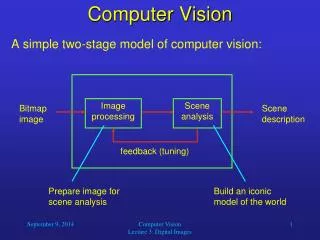
Image processing Sceneanalysis Bitmap image feedback (tuning) Prepare image for scene analysis Build an iconic model of the world Computer Vision • A simple two-stage model of computer vision: Scene description Computer Vision Lecture 3: Digital Images
Computer Vision • The image processing stage prepares the input image for the subsequent scene analysis. • Usually, image processing results in one or more new images that contain specific information on relevant features of the input image. • The information in the output images is arranged in the same way as in the input image. For example, in the upper left corner in the output images we find information about the upper left corner in the input image. Computer Vision Lecture 3: Digital Images
Computer Vision • The scene analysis stage interprets the results from the image processing stage. • Its output completely depends on the problem that the computer vision system is supposed to solve. • For example, it could be the number of bacteria in a microscopic image, or the identity of a person whose retinal scan was input to the system. • In the following lectures we will focus on the lower-level, i.e., image processing techniques. • Later we will discuss a variety of scene analysis methods and algorithms. Computer Vision Lecture 3: Digital Images
Computer Vision • How can we turn a visual scene into something that can be algorithmically processed? • Usually, we map the visual scene onto a two-dimensional array of intensities. • In the first step, we have to project the scene onto a plane. • This projection can be most easily understood by imagining a transparent plane between the observer (camera) and the visual scene. • The intensities from the scene are projected onto the plane by moving them along a straight line from their initial position to the observer. • The result will be a two-dimensional projection of the three-dimensional scene as it is seen by the observer. Computer Vision Lecture 3: Digital Images
(x, y, z) y’ y (x’, y’) z f x x’ Digitizing Visual Scenes • Obviously, any 3D point (x, y, z) is mapped onto a 2D point (x’, y’) by the following equations: Computer Vision Lecture 3: Digital Images
Actual Camera Geometry Computer Vision Lecture 3: Digital Images
Color Imaging via Bayer Filter Computer Vision Lecture 3: Digital Images
Magnetic Resonance Imaging Computer Vision Lecture 3: Digital Images
Digitizing Visual Scenes • In this course, we will mostly restrict our concept of images to grayscale. • Grayscale values usually have a resolution of 8 bits (256 different values), in medical applications sometimes 12 bits (4096 values), or in binary images only 1 bit (2 values). • We simply choose the available gray level whose intensity is closest to the gray value color we want to convert. Computer Vision Lecture 3: Digital Images
y’ [0, 0] [0, 1] [0, 2] [0, 3] [1, 0] [1, 1] [1, 2] [1, 3] [2, 0] [2, 1] [2, 2] [2, 3] x’ Digitizing Visual Scenes • With regard to spatial resolution, we will map the intensity in our image onto a two-dimensional finite array: Computer Vision Lecture 3: Digital Images
Digitizing Visual Scenes • So the result of our digitization is a two-dimensional array of discrete intensity values. • Notice that in such a digitized image F[i, j] • the first coordinate i indicates the row of a pixel, starting with 0, • the second coordinate j indicates the column of a pixel, starting with 0. • In an m×n pixel array, the relationship between image (with origin in ints center) and pixel coordinates is given by the equations Computer Vision Lecture 3: Digital Images
Image Size and Resolution Computer Vision Lecture 3: Digital Images
Intensity Resolution Computer Vision Lecture 3: Digital Images
Dithering Computer Vision Lecture 3: Digital Images
Floyd-Steinberg Dithering • The best dithering results are achieved by compensating for the thresholding error at a pixel x by adjusting the intensity of neighboring pixels. • Floyd-Steinberg dithering uses the following matrix for this purpose: Computer Vision Lecture 3: Digital Images
Levels of Computation • As we discussed before, computer vision systems usually operate at various levels of computation. • In the following, we will discuss different levels of computation as they occur during the image processing and scene analysis stages. • We will formalize this concept by means of an operation O that receives a set of pixels and returns a single intensity value that can be used to determine the value of a pixel in the output image. • We will look at operations at the point level, local level, global level, and object level mapping an input image FA[i, j] to an output image FB [i, j]. Computer Vision Lecture 3: Digital Images
Point Level • Operation type: • FB[i, j] = Opoint{FA[i, j]} • This means that the intensity of each pixel in the output image only depends on the intensity of the corresponding pixel in the input image. • Examples for this kind of operation are inversion (creating a negative image), thresholding, darkening, increasing brightness etc. Computer Vision Lecture 3: Digital Images
Local Level • Operation type: • FB[i, j] = Olocal{FA[k, l]; [k, l] N[i, j]} • Where N[i, j] is a neighborhood around the position [i, j]. For example, it could be defined as • N[i, j] = {[u, v] | |i – u| < 3 |j – v| < 3}. • Then the neighborhood would include all pixels within a 5×5 square centered at [i, j]. • So the intensity of each pixel in the output image depends on the intensity of pixels in the neighborhood of the corresponding position in the input image: • Examples: Blurring, sharpening. Computer Vision Lecture 3: Digital Images
Global Level • Operation type: • FB[i, j] = Oglobal{FA[k, l]; 0 ≤ k < m, 0 ≤ l < n} • for an m×n image. • So the intensity of each pixel in the output image may depend on the intensity of any pixel in the input image. • Examples: histogram modification, rotating the image Computer Vision Lecture 3: Digital Images
Object Level • The goal of computer vision algorithms usually is to determine properties of an image with regard to specific objects shown in it. • To do this, operations must be performed at the object level, that is, include all pixels that belong to a particular object. • Problem: We must use all points that belong to an object to determine its properties, but we need some of these properties to determine the pixels that belong to the object. • While this seems effortless in biological systems, we will later see that complex algorithms are required to solve this problem in an artificial system. Computer Vision Lecture 3: Digital Images


