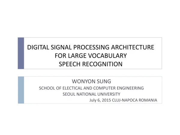
DIGITAL SIGNAL PROCESSING ARCHITECTURE FOR LARGE VOCABULARY SPEECH RECOGNITION
DIGITAL SIGNAL PROCESSING ARCHITECTURE FOR LARGE VOCABULARY SPEECH RECOGNITION. WONYON SUNG SCHOOL OF ELECTICAL AND COMPUTER ENGINEERING SEOUL NATIONAL UNIVERSITY July 6, 2015 CLUJ-NAPOCA ROMANIA. Speech recognition. Most natural human-machine interface.

DIGITAL SIGNAL PROCESSING ARCHITECTURE FOR LARGE VOCABULARY SPEECH RECOGNITION
E N D
Presentation Transcript
DIGITAL SIGNAL PROCESSING ARCHITECTURE FOR LARGE VOCABULARY SPEECH RECOGNITION WONYON SUNG SCHOOL OF ELECTICAL AND COMPUTER ENGINEERING SEOUL NATIONAL UNIVERSITY July 6, 2015 CLUJ-NAPOCA ROMANIA
Speech recognition • Most natural human-machine interface. • Long history of research (even from analog technology age) • Extensive use of DSP technology • Still imperfect • We nowadays understand it a kind of machine learning problems. • Diverse applications: Keyword spotting (~100 words) to multi-language understanding (> 100K words) One two three four …..
Hidden Markov model for speech recognition • Hidden Markov model contains states (tri-phone states) and state transitions according to the speech input and the network connections. It combines three knowledge sources. • Acoustic model – Phoneme representation, (Gaussian mixture model for emission probability computation) • Pronunciation model – vocabulary (lexicon) • Sentence or language model
HMM base speech recognition implementation Feature extraction: speech to acoustic parameter MFCC (Mel-Frequency Cepstrum Coefficient) Irrelevant of the vocabulary size Emission probability computation Generate the log-likelihood of each hypothesis state Higher dimension needed for large vocabulary (4 ~ 128th dimension) Viterbi beam search Dynamic programming through the network High complex ‘compare and select’ operations
Algorithm and implementation trend • ~ 2000 • Single CPU or programmable DSP based • ~ up to date • Hidden Markov model based • Parallel computer architecture (GPU, multi-core) • FPGA, VLSI • In the future • Neural network (deep neural network, recurrent neural network) • GPU, Neuromorphic system based In this talk: • Part1: multi-core CPU and GPU (parallel computer) based implementation of large vocabulary speech recognition • Part2: Deep neural network based implementations
Speech recognition for large vocabulary (>60K) • Not only lexicon size increases, more precise acoustic modeling: • High dimension (32~128) Gaussian mixture model • More tri-phone states • The network complexity for HMM grows very rapidly. • We need to prune many states or arcs during the search • Resulting in very irregular computation • High complexity language model needed: 3-gram or higher is desired. • Large memory size You, Kisun, et al. "Parallel scalability in speech recognition." Signal Processing Magazine, IEEE 26.6 (2009): 124-135.
... CAT ... HAT HOP IN ... ON POP ... THE ... ... CAT ... HAT HOP IN ... ON POP ... THE ... Recognition Network Example aa Features from one frame Gaussian Mixture Model for One Phone State HMM Acoustic Phone Model Pronunciation Model Mixture Components hh 17550 Triphones 128 Components 58k Word Vocabulary ... HOP hhaa p ... ON aa n ... POP p aa p ... … Computing distance toeach mixture components n … Computingweighted sumof all components Bigram Language Model • 4 million States • 10 millions Transition Arcs … … … … … … 168k Bigram Transitions Compiled & Optimized WFST Recognition Network
Multi-core CPU and GPU • Multicore: Two ~ 10’s CPU cores on each chip. Good single thread performance • GPU (manycore): 100’s of processing cores, maximizing computation throughput at the expense of single thread performance Intel Xeon Phi 96 cores NVIDIA GTX285 (55nm) 30 cores Intel Core i7 (45nm) 4 cores
Multicore/GPU Architecture Trends 4X32b • Increasing numbers of cores per die • Intel Nehalem: 4~8 cores • Intel Xeon Phi: about 60 cores • NVIDIA GTX285: 30 cores (each core contains 8 units) • Increasing vector unit width (SIMD) • Intel Core i7 (Nehalem): 8-way ~ 16-way • Intel Xeon Phi: 16-way • NVIDIA GTX285: 8-way (physical), 32-way (logical) a0 a1 a2 a3 b0 b1 b2 b3 + + + + a0+b0 a1+b1 a2+b2 a3+b3 Vector unit (SIMD) Core Core Core Core Core Core
Parallel scalability • Can we achieve the speed-up of ‘SIMD_width x #_of_cores’? • E.g. With 8-way SIMD, 8-core CPU, 64 times speed-up. • Some parts of speech recognition algorithm is quite parallel scalable, but other parts are not. • Emission probability computation: computation flow is quite regular. Good scalability • Hidden Markov network search: quite irregular network search • Packing overhead for SIMD • Synchronization overhead
Emission probability computation • Very regular and good candidate workload for parallelization • Tied HMM states (Senone) • Usually up to several thousands (depends on training condition) • 39 D MFCC feature vector • Gaussian mixture: 16, 32, 128 • Parallelization • Triphones (senone) for core-level • Gaussian for SIMD-level • Simple dynamic workload distribution • Count the number of active triphones • Distribute evenly to each thread
Irregular network search <-> parallel scalability Parallel graph traversal through an irregular network with millions of arcs and states • Vector (SIMD) unit efficiency • SIMD operation demands a packed data (packing overhead may be needed) • Continuously changing working set guided by input • Synchronization • Arc traversal induces write conflicts for destination state update • Increased chance of conflicts for large number of cores Core Core $ Core $ Core $ Core $ Core Synchronization Vector Unit Utilization $ Core $ HMMNetwork
Applying SIMD in network search j 1 a l Coalescing (gathering) data 8 10 12 g b 5 2 h Src state cost 2 3 4 8 k 9 11 c + 3 Arc Obs. Prob. b c d j d + i 6 4 Arc Weight b c d j e f < 7 Dest state cost 5 5 5 10 = Scattering data Updated Dest state cost 5 5 5 10
SIMD Efficiency ActiveStates Mapped onto SIMD SIMD Utilization Extra work Time
Parallelization choice of network search • Coarse grained vs fine grained job partitioning problem • Active-state or Active-arc based traversal • In this graph, (2) (3) (4) (8) for active state based parallelization. • In this graph, (b), (c), (d), (e) ..(j) for active arc based parallelization • Active-state based is simpler and coarse, but the number of arcs for each state varies • Active-arc based is fine-grained j 1 a l 8 10 12 g b 5 2 h k 9 11 c 3 d i 6 4 e f 7
Thread-scheduling issues • Assigning a destination node update to a single thread or multiple threads? • Minimum of incoming cost should be adopted (Viterbi) • Traversal by propagation • (2) (3) (4) are parallelized, the update of (5) can be done by multiple threads • Write-conflict problem • Atomic operation for the update • Privatization (Build private buffer) • Lock based implementation • Traversal by aggregation • (5) are update by a single thread • No write-conflict problem • Need preparation 1 Thread 0 5 2 3 Thread 1 6 4
Design Space for search network parallelization synch cost needed overhead needed coarse grain Current States Current States Current States Current States Next States Next States Next States Next States fine grain
Speedup: Multicore – relatively small # of cores Sequential RTF: 3.17; 1x State-based Propagation RTF: 0.925; 3.4x 3.4x speed-up with 4x4 = 16 times parallel hardware support RTF: Real Time Factor 3.4x: Speedup vsSeq Obs. Prob. Comp.Non-eps TraversalEps Traversal Seq. Overhead Arc-based Propagation RTF: 1.006; 3.2x State-based AggregationRTF: 2.593; 1.2x No SIMD in search!! Coalescing overhead exceeds 4-way SIMD benefit
Speedup: GPU – large number of cores Arc-based Propagation RTF: 0.302; 10.5x Sequential RTF: 3.17; 1x 10.5x speed-up with 240 (=8*30)parallel hardware support State-based Propagation RTF:0.776; 4.1x RTF: Real Time Factor 10.5x: Speedup vsSeq Obs. Prob. Comp.Non-eps TraversalEps Traversal Seq. Overhead Arc-based AggregationRTF: 0.912; 3.5x State-based AggregationRTF: 1.203; 2.6x Manycore
Conclusion for parallel speech recognition synch cost needed overhead needed Multi-core coarse grain Current States Current States Current States Current States Next States Next States Next States Next States fine grain Many-core or GPU
Part2 – speech recognition with deep neural network • Neural networks first used for speech recognition a few decades ago, but the performance was worse than GMM. • Single Hidden Layer • Lack of large data • Lack of processing power • Overfitting problem • Resurrection of neural network • Multiple Hidden Layers (deep neural network) • Large training sets are now available. • RBM pretraining reduces the overfitting problem. • NN returns with the name of Deep Neural Network and shows significantly better performance than GMM in phoneme recognition.
Deep neural network for acoustic modeling • Multiple layers of neural network • Each layer is (usually) all-to-all connection with activation function (e.g. sigmoid) • Considering that one layer contains 1,000 units, each layer demands 1 million weights, and 1 million multiply-add operations for one output computation • Five layer DNN implies 5 million (or 20 million with 2000 units) weights and operations a lot of memory and arithmetic operations Likelihood of phonemes
Strategies for low-power speech recognition systems • GPU based systems are not power efficient Approach for low-power • Do not use DRAM • All on-chip operations • Apply low voltage to lower the switching power (P = k C V2) • Parallel processing, instead of time-multiplexing • No global data transfer • Our solution • Use low-precision weights • All on-chip operations • Thousands of distributed processing units (no global communication)
DNN Implementation with fixed-point hardware • Reducing the precision of weights • For reduced memory size • For removing the multipliers • Retrain based fixed-point optimization of weights • Floating-point training • Step by step quantization from the 1st level to the last level • Retrain with quantized weights
Multiplier free, fully parallel DNN circuit • The resulting hardware (PU) employs no multipliers (adders and muxes) • Each layer contains 1K PUs. • With 1W, about 1000 times of real-time processing speed
Recurrent neural network (RNN) • Speech recognition needs sequence processing (memorizing past) • Delayed recurrent paths allow aneural network access theprevious inputs. • Long short-term memory (LSTM): special RNN structure that can learn very long time dependencies. • Recurrent • Feedforward
RNN for language model • Predict the next word/character when given the history of words/characters. • Input: one-hot encoded word/character, xt • Output: probabilities or confidences of the next words/characters e.g. P(xt+1|x1:t) for all xt+1 • Delayed recurrent pathsallow RNNs to accessthe previous inputs.
RNN-only speech recognition • CTC (connectionist temporal classification) objective function allows RNNs to learn sequences rather than frame-wise targets. • CTC only concerns the sequential order of the output labels, not the exact timing. • With CTC-based training, RNNs can directly learn to generate texts from speech data without any prior knowledge of the linguistic structures or dictionaries. • Long short-term memory (LSTM) RNN is used • Bidirectional architecture is employed to access the future input as well as the past input.
RNN-only speech recognition: results • Input: 39-dim MFCC feature (D_A_E) • Output: 29-dim characters, (a-z _ . ’) • Network topology:- 3 BLSTM layers, 256 memory blocks per LSTM layer, 3.8 M weights • Training data: WSJ0 + WSJ1 + TIMIT training set (66,319,215 frames), about 1 month training with a single thread CPU. • Test data: TIMIT complete test set • Character error rate 17.94 % • w e l l _ j u n i o r _ d i d n ' t _ h e _ e a t _ o n l y _ o n e _ a n d _ m r _ h e n r y _ d i d n ' t _ e v e n _ d o _ t h a t _ w e l l _w e l _ j u n o r _ d i d n ' t _ h e _ e a t _ o n l y _ o n e _ a n d _ m r . _ h e n r y _ d i d n ' t _ e v e n _ d o _ t h a t _ w e l l _(Word-level learning)e t e r n i t y _ i s _ n o _ t i m e _ f o r _ r e c r i m i n a t i o n s _a u t t o r n i t y _ i s _ n o _ t i m e _ f o r _ r e c r i m i n a t i o n s _(The word “recrimination” is not in the training set)l a u g h _ d a n c e _ a n d _ s i n g _ i f _ f o r t u n e _ s m i l e s _ u p o n _ y o u _l a f h _ d a n c e _ a n d _ s i n g _ o _ f o r t u n e _ s m i l e _ s u p p o n y o u _
Characteristics of DNN (& RNN) bases speech recognition Disadvantages: Large number of weights, large number of arithmetic operations Many advantages leading to low-power consumption • Highly paralleland regular (most operations are inner product of 512 ~ 2K inputs) computation • Non-volatile memory can be used for recognition only (off-line training) architecture, • High density (10 times of SRAM), low power, no standing-by power • Low precision arithmetic: DNN architecture is very robust to quantization when quantization is included in the training procedure • Weight memory saving, arithmetic unit size reduction • Thousands of distributed arithmetic units • Mostly local connection
Conclusion Architectural trends for speech recognition
References • You, Kisun, et al. "Parallel scalability in speech recognition." Signal Processing Magazine, IEEE 26.6 (2009): 124-135. • Choi, Y. K., You, K., Choi, J., & Sung, W. (2010). A real-time FPGA-based 20 000-word speech recognizer with optimized DRAM access. Circuits and Systems I: Regular Papers, IEEE Transactions on, 57(8), 2119-2131. • Graves, Alex, and NavdeepJaitly. "Towards end-to-end speech recognition with recurrent neural networks." Proceedings of the 31st International Conference on Machine Learning (ICML-14). 2014. • Hwang, Kyuyeon, and Wonyong Sung. "Fixed-point feedforward deep neural network design using weights+ 1, 0, and− 1." Signal Processing Systems (SiPS), 2014 IEEE Workshop on. IEEE, 2014.