New Product Development
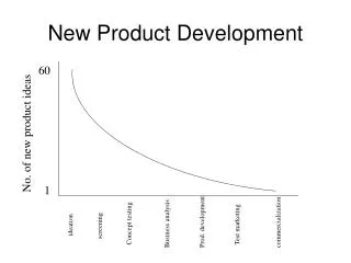
New Product Development. Sales Forecasting & Financial Analysis. Sales Forecasts. With Sales Potential Estimates. Mail Concept Test – Drawing / Diagram. Sales Potential Estimation. Translating Intent into Sales Potential


New Product Development
E N D
Presentation Transcript
New Product Development Sales Forecasting & Financial Analysis
Sales Forecasts • With Sales Potential Estimates
Sales Potential Estimation • Translating Intent into Sales Potential • Example: Aerosol Hand CleanerAfter examining norms for comparable existing products, you determine that: • 90% of the “definites” • 40% of the “probables” • 10% of the “mights” • 0% of the “probably nots” and “definitely nots”will actually purchase the product • Apply those %age to Concept Test results:
Sales Potential Estimation • Translating Intent into Sales Potential • Apply those %age to Concept Test results: • 90% of the “definites” (5% of sample) = .045 • 40% of the “probables” (36%) = .144 • 10% of the “mights” (33%) = .033 • 0% of the last 2 categories = .000 • Sum them to determine the %age who would actually buy: .045+.144+.033= .22 • Thus, 22% of sample population would buy(remember: this % is conditioned on awareness & availability)
From Potential to Forecast • With Sales Potential Estimates: • To remove the conditions of awareness and availability, multiply by the appropriate percentages: • If 60% of the sample will be aware (via advertising, etc.) and the product will be available in 80% of the outlets, then: • (.22) X (.60) X (.80) = .11 • 11% of the sample is likely to buy
Sales Forecasts • With Sales Potential Estimates • Diffusion of Innovations • The Bass Model: • Predicts pattern of trial (doesn’t include repeat purchases) at the category level • Works for all types of products, and can be used with discontinuous innovations
The Bass Model • Estimates s(t) = sales of the product class at some future time t:s(t) = pm + [q-p] Y(t) - (q/m) [Y(t)]2Wherep = the “coefficient of innovation” [Average value=.04]q = the “coefficient of imitation” [Average value =.30]m= the total number of potential buyersY(t) = the total number of purchases by time t
The Bass Model • Important Feature • Once p and q have been estimated, you can determine the time required to hit peak sales (t*) • and the peak sales level at that time (s*):t* = (1/(p+q)) ln (q/p) s* = (m)(p+q)2/4q
Financial Analysis • How Sophisticated? • Depends on the quality/reliability of the data and the stage you’re in • Early Stages: • Simple cost/benefit analysis or • “Sanity Check” as 3M uses: • attractiveness index = (sales X margin X(life).5 ) / cost • sales= likely sales for “typical year” once launchedmargin = likely margin (in percentage terms)life = expected life of the product in years (sq root discounts future)cost = cost of getting to market (dev., launch, cap.ex.)
Financial Analysis: Later Stages • Payback and Break-Even Times • Cycle Time • Payback Period • Break-Even Time (BET) = Cycle Time + Payback Pd.
Financial Analysis: Later Stages • Payback and Break-Even Times
Financial Analysis: Later Stages • Payback and Break-Even Times • Discounted Cash Flows (DCF, NPV, or IRR) • The most rigorous analysis for new products: • year-by-year cash flow projections discounted to the present • the discounted cash flows are summed • if the sum of the dcf’s > initial outlays, the project passes • The “Dark Side” of NPV (for NPD) • Unfairly penalizes certain projects by ignoring the Go/Kill options along the way (option values not accounted for in traditional NPV)
Financial Analysis: Later Stages • Payback and Break-Even Times • Discounted Cash Flows (DCF, NPV, or IRR) • Options Pricing Theory (OPT) • Recognizes that management can kill a project after an incremental investment is made • At each phase of the NPD process, management is effectively “buying an option” on the project • These options cost considerably less than the full cost of the project -- so they are effective in reducing risk • Kodak uses a decision tree and uses OPT to compute the Expected Commercial Value (ECV) of a given project
Using OPT to find the ECV Commercial Success $PVI Pcs Technical Success Yes Launch $C Pts Yes No Development $D Commercial Failure $ECV No Technical Failure KEY: Pts = Prob of tech success $D = Development costs remaining Pcs= Prob of comm success $C = Commercialization/launch costs $ECV = Expected commercial value $PVI = Present value of future earnings
Using OPT to find the ECV ECV = [ [(PVI * Pcs) - C] * Pts] - D KEY: Pts = Prob of tech success $D = Development costs remaining Pcs= Prob of comm success $C = Commercialization/launch costs $ECV = Expected commercial value $PVI = Present value of future earnings
NPV vs. OPT: An Example Income stream, PVI (present valued) $40 million Commercialization costs (launch & captial) $ 5 million Development costs $ 5 million Probability of commercial success 50% Probability of technical success 50% Overall probability of success 25% TRADITIONAL NPV (no probabilities): 40 - 5 - 5 = 30 Decision = Go NPV with probabilities: (.25 X 30) - (.75 X 10) = 0 Decision = Kill ECV or OPT: { [(40 x .5) - 5] * .5} - 5 = 2.5 Decision = Go