Poisson Processes
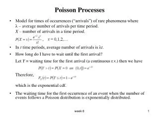
Poisson Processes. Model for times of occurrences (“arrivals”) of rare phenomena where λ – average number of arrivals per time period. X – number of arrivals in a time period. In t time periods, average number of arrivals is λ t . How long do I have to wait until the first arrival?

Poisson Processes
E N D
Presentation Transcript
Poisson Processes • Model for times of occurrences (“arrivals”) of rare phenomena where λ – average number of arrivals per time period. X – number of arrivals in a time period. • In t time periods, average number of arrivals is λt. • How long do I have to wait until the first arrival? Let Y = waiting time for the first arrival (a continuous r.v.) then we have Therefore, which is the exponential cdf. • The waiting time for the first occurrence of an event when the number of events follows a Poisson distribution is exponentially distributed. week 6
Expectation • In the long run, rolling a die repeatedly what average result do you expact? • In 6,000,000 rolls expect about 1,000,000 1’s, 1,000,000 2’s etc. Average is • For a random variable X, the Expectation (or expected value or mean) of Xis the expected average value of X in the long run. • Symbols: μ, μX, E(X) and EX. week 6
Expectation of discrete random variable • For a discrete random variable X with pmf whenever the sum converge absolutely . week 6
Examples 1) Roll a die. Let X = outcome on 1 roll. Then E(X) = 3.5. 2) Bernoulli trials and . Then 3) X ~ Binomial(n, p). Then 4) X ~ Geometric(p). Then 5) X ~ Poisson(λ). Then week 6
Expectation of continuous random variable • For a continuous random variable X with density whenever this integral converge absolutely. week 6
Examples 1) X ~ Uniform(a, b). Then 2) X ~ Exponential(λ). Then 3) X is a random variable with density (i) Check if this is a valid density. (ii) Find E(X) week 6
4) X ~ Gamma(α, λ). Then 5) X ~ Beta(α, β). Then week 6
Theorem For g: RR • If X is a discrete random variable then • If X is a continuous random variable • Proof: We proof it for the discrete case. Let Y = g(X) then week 6
Example to illustrate steps in proof • Suppose i.e. and the possible values of X are so the possible values of Y are then, week 6
Examples 1. Suppose X ~ Uniform(0, 1). Let then, 2. Suppose X ~ Poisson(λ). Let , then week 6
Properties of Expectation For X, Y random variables and constants, • E(aX + b) = aE(X) + b Proof: Continuous case • E(aX + bY) = aE(X) + bE(Y) Proof to come… • If X is a non-negative random variable, then E(X) = 0 if and only if X = 0 with probability 1. • If X is a non-negative random variable, then E(X) ≥ 0 • E(a) = a week 6
Moments • The kth moment of a distribution is E(Xk). We are usually interested in 1st and 2nd moments (sometimes in 3rd and 4th) • Some second moments: 1. Suppose X ~ Uniform(0, 1), then 2. Suppose X ~ Geometric(p), then week 6
Variance • The expected value of a random variable E(X) is a measure of the “center” of a distribution. • The variance is a measure of how closely concentrated to center (µ) the probability is. It is also called 2nd central moment. • Definition The variance of a random variable X is • Claim: Proof: • We can use the above formula for convenience of calculation. • The standard deviation of a random variable X is denoted by σX ; it is the square root of the variance i.e. . week 6
Properties of Variance For X, Y random variables and are constants, then • Var(aX + b) = a2Var(X) Proof: • Var(aX + bY) = a2Var(X) + b2Var(Y) + 2abE[(X – E(X ))(Y – E(Y ))] Proof: • Var(X) ≥ 0 • Var(X) = 0 if and only if X = E(X) with probability 1 • Var(a) = 0 week 6
Examples 1. Suppose X ~ Uniform(0, 1), then and therefore 2. Suppose X ~ Geometric(p), then and therefore 3. Suppose X ~ Bernoulli(p), then and therefore, week 6
Example • Suppose X ~ Uniform(2, 4). Let . Find . • What if X ~ Uniform(-4, 4)? week 6