Signals and Systems.

1. CHAPTER 1 Signals and Systems. School of Computer and Communication Engineering, UniMAP PuanNordianaBintiMohamadSaaid dianams@unimap.edu.my EKT 230

2. Signals and Systems. 1.1 What is a Signal ? 1.2 Classification of a Signals. 1.2.1 Continuous-Time and Discrete-Time Signals 1.2.2 Even and Odd Signals. 1.2.3 Periodic and Non-periodic Signals. 1.2.4 Deterministic and Random Signals. 1.2.5 Energy and Power Signals. 1.3 Basic Operation of the Signal. 1.4 Elementary Signals. 1.4.1 Exponential Signals. 1.4.2 Sinusoidal Signal. 1.4.3 Sinusoidal and Complex Exponential Signals. 1.4.4 Exponential Damped Sinusoidal Signals. 1.4.5 Step Function. 1.4.6 Impulse Function. 1.4.7 Ramped Function.

3. Cont’d… 1.5 What is a System ? 1.5.1 System Block Diagram. 1.6 Properties of the System. 1.6.1 Stability. 1.6.2 Memory. 1.6.3 Causality. 1.6.4 Inevitability. 1.6.5 Time Invariance. 1.6.6 Linearity.

4. 1.1 What is a Signal ? • A common form of human communication; (i) use of speechsignal, face to face or telephone channel. (ii) use of visual signal, taking the form of images of people or objects around us. • Real life examplesof signals; (i) Doctor listening to the heartbeat, blood pressure and temperature of the patient. These represent signals that conveys information about the state of health of the patient. (ii) Weather forecast provides information on the temperature, humidity, and the speed and direction of the prevailing wind. The signals represented by these quantities help us decide whether to stay indoor or doing some outdoor activity. • Indeed , the list of what constitutes a signal is almost endless.

5. Cont’d… • By definition,signal is a function of one or more variable that conveys information on the nature of a physical phenomenon. • When the function depends on a single variable, the signal is said to be one dimensional. Example of one dimensional signal: A speech signal whose amplitude varies with time, depending on the spoken word and who speaks it. • When the function depends on two or more variables, the signal is said to be multidimensional. Example of multidimensional signal: An image with horizontal and vertical coordinates of the image representing the two dimensions.

6. 1.2 Classifications of a Signal. • There are five types of signals; (i) Continuous-Time and Discrete-Time Signals (ii) Even and Odd Signals. (iii) Periodic and Non-periodic Signals. (iv) Deterministic and Random Signals. (v) Energy and Power Signals.

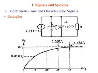
7. 1.2.1 Continuous-Time and Discrete-Time Signals. Continuous-Time (CT) Signals • Continuous-Time (CT) Signals are functions whose amplitude or value varies continuously with time, x(t). • The symbol tdenotes time for continuous-time signal and ( ) used to denote continuous-time value quantities. • Example: microphone converts variation in sound pressure (e.g speech) into corresponding variation in voltage and current. Figure 1.1: Continuous-Time Signal, x(t).

8. Cont’d… Discrete-Time Signals • Discrete-Time Signalis defined only at discrete instants of time. Thus, the independent variable has discrete values only, which are usually uniformly spaced. • It is often derived from continuous-time signal by sampling it at a uniform rate. Let Ts denote the sampling period and n denote an integer. The symbol n denotes time for discrete time signal and [ ] is used to denote discrete-value quantities. Figure 1.12 (a) Continuous-time signal x(t) . b) Representation of x(t) as a discrete-time signal.

9. 1.2.2 Even and Odd Signals. • A continuous-time signal x(t) is said to be an even signal if • The signal x(t) is said to be an oddsignal if • In summary, an evensignal are symmetric about the vertical axis (time origin) whereas an odd signal are antisymetric about the origin. Figure 1.4: Even Signal Figure 1.5: Odd Signal.

10. Example : Even and Odd Signals Suppose we are given an arbitrary signal x(t). x(t)is a sum of two components of , which is even function and , which is odd function. For even signal, For odd signal, Putting t = -t in the expression for x(t), we may write, Solving for and , we thus obtain, and

11. Cont’d…

12. Example 1.1: Even and Odd Signals. Find the even and odd components of each of the following signals: • x(t) = 4cos(3πt) Answer: ge(t) = 4cos(3πt) go(t) = 0

13. 1.2.3 Periodic and Non-Periodic Signals. Periodic Signal. • A periodic signal x(t) is a function of time that satisfies the condition where T is a positive constant. • The smallest value of T that satisfy the definition is called a period. Figure 1.6: Aperiodic Signal. Figure 1.7: Periodic Signal.

14. 1.2.4 Deterministic and Random Signals. Deterministic Signal. • A deterministic signal is a signal that is no uncertainty with respect to its value at any time. • The deterministic signal can be modeled as completely specified function of time. Figure 1.8: Deterministic Signal; Square Wave.

15. Cont’d… Random Signal. • A random signal is a signal about which there is uncertainty before it occurs. The signal may be viewed as belonging to an ensemble or a group of signals which each signal in the ensemble having a different waveform. • The signal amplitude fluctuates between positive and negative in a randomly fashion. • Example; noise generated by amplifier of a radio or television. Figure 1.9: Random Signal

16. 1.2.5 Energy Signal and Power Signals. Energy Signal. • A signal is refer to energy signal if and only if the total energy satisfy the condition; Power Signal. • A signal is refer to power signal if and only if the average power of signal satisfy the condition;

17. 1.2.6 Bounded and Unbounded Signals. Figure 1.10: Bounded and Unbounded Signal

18. 1.3 Basic Operation of the Signals. 1.3.1 Time Scaling. 1.3.2 Reflection and Folding. 1.3.3 Time Shifting. 1.3.4 Precedence Rule for Time Shifting and Time Scaling.

19. 1.3.1 Time Scaling. • Time scaling refers to the multiplication of the variable by a real positive constant. • If a > 1 the signal y(t) is a compressedversion of x(t). • If 0 < a < 1 the signal y(t) is an expandedversion of x(t). • Example: Figure 1.11: Time-scaling operation; continuous-time signal x(t), (b) version of x(t) compressed by a factor of 2, and (c) version of x(t) expanded by a factor of 2.

20. Cont’d… • In the discrete time, • It is defined for integer value of k, k > 1. Figure below for k = 2, sample for n = +-1, Figure 1.12: Effect of time scaling on a discrete-time signal: (a) discrete-time signal x[n] and (b) version of x[n] compressed by a factor of 2, with some values of the original x[n] lost as a result of the compression.

21. 1.3.2 Reflection and Folding. • Let x(t) denote a continuous-time signal and y(t) is the signal obtained by replacing time t with –t; • y(t) is the signal represents a reflected version of x(t) about t = 0. • Two special casesfor continuous and discrete-time signal; (i) Even signal; x(-t) = x(t) an even signal is same as reflected version. (ii) Odd signal; x(-t) = -x(t) an odd signal is the negative of its reflected version.

22. Example 1.2:Reflection. Given the triangular pulse x(t), find the reflected version of x(t) about the amplitude axis (origin). Solution: Replace the variable t with –t, so we get y(t) = x(-t) as in figure below. Figure 1.13: Operation of reflection: (a) continuous-time signal x(t) and (b) reflected version of x(t) about the origin x(t) = 0 for t < -T1 and t > T2. y(t) = 0 for t > T1 and t< -T2. • .

23. 1.3.3 Time Shifting. • A time shift delayor advances the signal in time by a time interval +t0 or –t0, without changing its shape. y(t) = x(t - t0) • If t0 > 0 the waveform of y(t) is obtained by shifting x(t) toward the right, relative to the time axis. • If t0< 0, x(t) is shifted to the left. Example: Figure 1.14: Shift to the Left. Figure 1.15: Shift to the Right. Q: How does the x(t) signal looks like?

24. Example 1.3: Time Shifting. Given the rectangular pulse x(t) of unit amplitude and unit duration. Find y(t)=x (t - 2) Solution: t0 is equal to 2 time units. Shift x(t) to the right by 2 time units. Figure 1.16: Time-shifting operation: • continuous-time signal in the form of a rectangular pulse of amplitude 1.0 and duration 1.0, symmetric about the origin; and (b) time-shifted version of x(t) by 2 time shifts. • .

25. 1.3.4 Precedence Rule for Time Shifting and Time Scaling. • Time shiftingoperation is performed first on x(t), which results in • Time shift has replace t in x(t) by t - b. • Time scaling operation is performed on v(t), replacing t by at and resulting in, • Example in real-life: Voice signal recorded on a tape recorder; • (a > 1) tape is played faster than the recording rate, resulted in compression. • (a < 1) tape is played slower than the recording rate, resulted in expansion.

26. Example 1.4:Continuous Signal. A CT signal is shown in Figure 1.17 below, sketch and label each of this signal; a) x(t-1) b) x(2t) c) x(-t) Figure 1.17 x(t) 2 t -1 3

27. x(-t) 2 t -3 1 • Solution: • (a) x(t-1) (b) x(2t) • (c) x(-t) x(t) x(t-1) 2 2 t t 0 4 -1/2 3/2

28. x[n] 4 2 0 1 2 3 n Example 1.5: Discrete Time Signal. A discrete-time signal x[n] is shown below, Sketch and label each of the following signal. (a) x[n – 2] (b) x[2n] (c.) x[-n+2] (d) x[-n]

29. Cont’d… x[n-2] 4 2 0 1 2 3 4 5 n (a) A discrete-time signal, x[n-2]. • A delay by 2

30. Cont’d… x(2n) 4 2 0 1 2 3 n (b) A discrete-time signal, x[2n]. Time scaling by a factor of 2.

31. Cont’d… x(-n+2) 4 2 -1 0 1 2 n (c) A discrete-time signal, x[-n+2]. Time shifting and reflection

32. Cont’d… x(-n) 4 2 -3 -2 -1 0 1 n (d) A discrete-time signal, x[-n]. • Reflection

33. x(t) 4 0 4 t In Class Exercises . A continuous-time signal x(t) is shown below, Sketch and label each of the following signal (a) x(t – 2) (b) x(2t) (c.) x(t/2) (d) x(-t)

34. 1.4 Elementary Signals. • There are many types of signals prominently used in the study of signals and systems. 1.4.1 Exponential Signals. 1.4.2 Exponential Damped Sinusoidal Signals. 1.4.3 Step Function. 1.4.4 Impulse Function. 1.4.5 Ramp Function.

35. 1.4.1 Exponential Signals. • A real exponential signal, is written as x(t) = Beat. • Where both B and a are real parameters. B is the amplitude of the exponential signal measured at time t = 0. (i) Decaying exponential, for which a < 0. (ii) Growing exponential, for which a > 0. Figure 1.18: (a) Decaying exponential form of continuous-time signal. (b) Growing exponential form of continuous-time signal. Figure 1.19: (a) Decaying exponential form of discrete-time signal. (b) Growing exponential form of discrete-time signal.

36. Cont’d… Continuous-Time. • Case a = 0: Constant signal x(t) =C. • Case a > 0: The exponential tends to infinity as tinfinity. Case a > 0 Case a < 0 • Case a < 0: The exponential tend to zero as tinfinity • (here C > 0).

37. Cont’d… Discrete-Time. where B and a are real. There are six cases to consider apart from a = 0. • Case 1 (a = 0): Constant signal x[n]=B. • Case 2 (a > 1): positive signal that grows exponentially. • Case 3 (0 < a < 1): The signal is positive and decays exponentially.

38. Cont’d… • Case 4 (a < 1): The signal alternates between positive and negative values and grows exponentially. • Case 5 (a = -1): The signal alternates between +C and -C. • Case 6 (-1 < a <0): The signal alternates between positive and negative values and decays exponentially.

39. 1.4.2 Sinusoidal Signals. • A general form of sinusoidal signal is • where A is the amplitude, wo is the frequency in radians per second, and q is the phase angle in radians. Figure 1.20: Continuous-Time Sinusoidal signal A cos(ω0t + θ).

40. Cont’d… • Discrete time version of sinusoidal signal, written as Figure 1.21: Discrete-Time Sinusoidal Signal A cos(ωt + Φ).

41. 1.4.3 Sinusoidal and Complex Exponential Signals. • Complex exponential, • Euler’s Identity, • Complex exponential signal, • Where, • Hence, • Thus, in terms of real and imaginary parts;

42. 1.4.3 Sinusoidal and Complex Exponential Signals. • Continuous time sinusoidal signals, • In the discrete time case,

43. Cont’d… Figure 1.22: Complex plane, showing eight points uniformly distributed on the unit circle.

44. 1.4.4 Exponential Damped Sinusoidal Signals. • Multiplication of a sinusoidal signal by a real-value decaying exponential signal result in an exponential damped sinusoidal signal. • Where ASin(wt + f) is the continuous signal and e-at is the exponential Figure 1.23: Exponentially damped sinusoidal signal Ae-at sin(ωt), with A = 60 and α = 6. • Observe that in Figure 1.23, an increased in time t, the amplitude of the sinusoidal oscillation decrease in an exponential fashion and finally approaching zero for infinite time.

45. 1.4.5 Step Function. • The discrete-time version of the unit-step function is defined by, Figure 1.24: Discrete–time of Step Function of Unit Amplitude.

46. Cont’d… • The continuous-time version of the unit-step function is defined by, Figure 1.25: Continuous-time of step function of unit amplitude. • The discontinuity exhibit at t = 0 and the value of u(t) changes instantaneously from 0 to 1 when t = 0. That is the reason why u(0) is undefined.

47. 1.4.6 Impulse Function. • The discrete-time version of the unit impulse is defined by, Figure 1.26: Discrete-Time form of Impulse. • Figure 1.41 is a graphical description of the unit impulse d(t). • The continuous-time version of • the unit impulse is defined by • the following pair, • The d(t) is also refer as the Dirac Delta function.

48. Cont’d… • Figure 1.27 is a graphical description of the continuous-time unit impulse d(t). Figure 1.27: (a) Evolution of a rectangular pulse of unit area into an impulse of unit strength (i.e., unit impulse). (b) Graphical symbol for unit impulse. (c) Representation of an impulse of strength a that results from allowing the duration Δ of a rectangular pulse of area a to approach zero. • The duration of the pulse, (t) decreased and its amplitude is increased. The area under the pulse is maintained constant at unity.

49. Cont’d…

50. 1.4.7 Ramp Function. • The integral of the step function u(t) is a ramp function of unit slope. or Figure 1.28: Ramp Function of Unite Slope. • The discrete-time version of the ramp function, Figure 1.29: Discrete-Time Version of the Ramp Function.