Download

1 / 32
320 likes | 552 Vues
Outline. ContextSpace time models for disease riskUse of space time models to investigate the stability of patterns of diseaseIllustration on the analysis of congenital malformationsIllustration on the analysis of bladder cancer in UtahDiscussion. . Benefits of Space Time Analysis for chronic d

E N D
3. Benefits of Space Time Analysis for chronic diseases Study the persistence of patterns over time
Interpreted as associated with stable risk factors, environmental effects, distribution of health care access �
Highlight unusual patterns in time profiles via the inclusion of space-time interaction terms
Time localised excesses linked to e.g. emerging environmental hazards with short latency
Variability in recording practices
Increased epidemiological interpretability
Potential tool for surveillance
4. Case study: Congenital anomalies in England All cases of congenital anomalies (non chromosomal) recorded in England for the period 1983 � 1998
Data from national post-coded registers (Office for National Statistics)
Annual post-coded data on total number of live births, still births and terminations
136,000 congenital anomalies ? 84.5 per 105 birth-years
Congenital anomalies are sparse:
? Grid of 970 grid squares with variable size, to equalize the number of birth and expected cases per square
Variations could be linked to socio-economic or environmental risk factors or heterogeneity in recording practises
? Interest in characterising space time patterns
7. Case study: Bladder cancer Bladder cancer incidence in Utah (US), 1973-2004
Spatial resolution: census tracts (496)
Between 0 and 11 new cases per year with mean around 0.4
Time periods: 1973-76, 1977-80,�, 2001-04
Expected counts based on sex-age incidence rates for the region and the total period 1973-2004
8. Case study: Bladder cancer
11. Schematic representation
14. Prior structure for the random effects Overall spatial pattern: account for local dependence due to geographical �continuity� of populations and risk factors
use �spatial autoregressive model� commonly employed for disease mapping
Overall time trends: time dependence might be expected, e.g.for long latency chronic diseases use � time structured autoregressive model�
Space time interactions: capture the non predictable part from simple space + time model
what model to use ?
15. New model for the interaction terms Investigating stability of patterns: Aim is to
-- Highlight true departures from the overall predictable �space + time� model
the variance of nit has to be allowed to be large
-- Shrink idiosynchratic (non interpretable) interactions: small variance for most nit
? Mixture model to characterise �stable� and �unstable� risk patterns over time
17. Analysis strategy for investigating stability of patterns Estimate a model:
space + time + interactions (mixture)
Use the posterior probabilities of allocation pit into component 2 to classify areas as �unstable�
Rule: area i is unstable if at least for one t, pit is large, i.e. pit > pcut (threshold probability). Other rules possible
For �stable� areas, investigate spatial patterns, e.g. by using the rule Prob(exp(?i ) >1) > 0.8.
Investigate the time profile pattern of �unstable� areas
22. Mixture estimation Using a cut off
pcut = 0.5, 125 areas (13%) are classified as unstable
23. Risk time profiles for the areas classified as unstable
24. Bladder cancer, Utah, 1973-2004 Spatial main effect (496 Census Tracts)
Posterior median of exp(?i) = spatial RR Linda va faire une nouvelle carte avec dans la 1ere classe les 96 R spatiaux elev�s et dans la derniere classe les 81 R spatiaux bas. Les 3 census tracts avec des R spatiaux elev�s et non persistants auront une croixLinda va faire une nouvelle carte avec dans la 1ere classe les 96 R spatiaux elev�s et dans la derniere classe les 81 R spatiaux bas. Les 3 census tracts avec des R spatiaux elev�s et non persistants auront une croix
25. Bladder cancer, Utah, 1973-2004 Time main effects
Posterior median of exp(?t) = Temporal RR
26. Bladder cancer, Utah, 1973-2004 Posterior distribution of ?1 and ?2
27. Bladder cancer, Utah, 1973-2004 Census tracts classified as �unstable� using
the rule pit >0.6
28. Bladder cancer, Utah, 1973-2004 Space-time interactions for the 13 areas classified as �unstable�
29. Bladder cancer, Utah, 1973-2004