Download
1 / 25
250 likes | 274 Vues
This study presents a comprehensive analysis of solar wind and interplanetary disturbances using analytic, empirical, and numerical models. It explores the evolution of density structures and the appearance of transient density structures in synthetic white-light imaging. The interaction between the disturbances and the ambient solar wind is also examined. The study provides important insights into the propagation and behavior of interplanetary shocks and coronal mass ejections.

E N D
State of NOAA-SEC/CIRES STEREO Heliospheric Models Dusan Odstrcil University of Colorado/CIRES & NOAA/Space Environment Center STEREO SWG Meeting, NOAA/SEC, Boulder, CO, March 22, 2004
Nick Arge – AFRL, Hanscom, MA • Chris Hood – University of Colorado, Boulder, CO • Jon Linker – SAIC, San Diego, CA • Rob Markel – University of Colorado, Boulder, CO • Leslie Mayer – University of Colorado, Boulder, CO • Vic Pizzo – NOAA/SEC, Boulder, CO • Pete Riley – SAIC, San Diego, CA • Marek Vandas – Astronomical Institute, Prague, Czech Republic • Xuepu Zhao – Stanford University, Standford, CA Collaborators Supported by AFOSR/MURI and NSF/CISM projects
Input Data • Analytic Models: - structured solar wind (bi-modal, tilted) - over-pressured plasma cloud (3-D) - magnetic flux-rope (3-D in progress) • Empirical Models: - WSA source surface - SAIC source surface - CME cone model (location, diameter, and speed) • Numerical Models: - SAIC coronal model (ambient + transient outflow)
Numerical Model -- Magnetic Flux Rope Shock Model Interface Ejected Plasma Magnetic Leg Compressed Plasma
Ambient Solar Wind Models CU/CIRES-NOAA/SEC 3-D solar wind model based on potential and current-sheet source surface empirical models SAIC 3-D MHD steady state coronal model based on photospheric field maps [ SAIC maps – Pete Riley ] [ WSA maps – Nick Arge ]
CME Cone Model Best fitting for May 12, 1997 halo CME • latitude: N3.0 • longitude: W1.0 • angular width: 50 deg • velocity:650 km/s at 24 Rs (14:15 UT) • acceleration: 18.5 m/s2 [ Zhao et al., 2001 ]
Boundary Conditions Ambient Solar Wind + Plasma Cloud Ambient Solar Wind
Latitudinal Distortion of ICME Shape ICME propagates into bi-modal solar wind
Evolution of Density Structure ICME propagates into the enhanced density of a streamer belt flow
Appearance of Transient Density Structure IPS observations detect interplanetary transients that sometime show two enhanced spots instead of a halo ring [Tokumaru et al., 2003] MHD simulation shows a dynamic interaction between the ICME and ambient solar wind that: (1) forms an arc-like density structure; and (2) results in two brighter spots in synthetic images
May 12, 1997 – Interplanetary Shock Distribution of parameters in equatorial plane Evolution of velocity on Sun-Earth line 0.2 AU 0.4 AU 0.6 AU 0.8 AU • Shock propagates in a fast stream and • merges with its leading edge 1.0 AU
Case A1 Case A3 [ SAIC maps -- Pete Riley ] Fast-Stream Position Ambient state before the CME launch Disturbed state during the CME launch Ambient state after the CME launch
[ SAIC maps -- Pete Riley ] Effect of Fast-Stream Position Case A1 Case A3 Earth : Interaction region followed by shock and CME (not observed) Earth : Shock and CME (observed but 3-day shift is too large)
Case A2 Case B2 [ SAIC maps -- Pete Riley ] Fast-Stream Evolution Ambient state before the CME launch Disturbed state during the CME launch Ambient state after the CME launch
[ SAIC maps -- Pete Riley ] Effect of Fast-Stream Evolution Case A2 Case B2 Earth : Interaction region followed by shock and CME (not observed) Earth : Shock and CME (observed but shock front is radial)
Client Server Coronal Data (on MSS) Remote Access ENKI -- web ENKI IDL procedures Input Data (on PTMP) ENLIL – Fortran/MPI/NetCDF A/A – Java/VTK ViServer Output Data (on PTMP) web CDP Archive Data (on MSS)
Remote Visualization: ENKI--IDL Preview of data before downloading processing and visualization, archiving, etc. Plot 1-D profiles and 2-D contours or surfaces of 1-D, 2-D, or 3-D data