Download

1 / 55
580 likes | 950 Vues
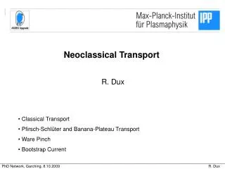
Neoclassical Transport. R. Dux. Classical Transport Pfirsch-Schlüter and Banana-Plateau Transport Ware Pinch Bootstrap Current. Why is neoclassical transport important?. Usually, neoclassical (collisional) transport is small compared to the turbulent transport.

E N D
Neoclassical Transport R. Dux • Classical Transport • Pfirsch-Schlüter and Banana-Plateau Transport • Ware Pinch • Bootstrap Current
Why is neoclassical transport important? • Usually, neoclassical (collisional) transport is small compared to the turbulent transport. • Neoclassical transport is important: • when turbulent transport becomes small - transport barriers (internal, edge barrier in H-modes) - central part of the plasma, where gradients are small • to understand the bootstrap current and the plasma conductivity • transport in a stellarator (we do not cover this)
Transport of particles, energy …due to collisions The gradients of density, temperature and electric potential in the plasma disturb the Maxwellian velocity distribution of the particles, which would prevail in thermodynamic equilibrium. The disturbance shall be small. Coulomb collisions cause friction forces between the different species and drive fluxes of particles and energy in the direction of the gradients. Coulomb collisions drive the velocity distribution towards the local thermodynamic equilibrium and the fluxes try to diminish the gradients. We seek for linear relations between the fluxes and the thermodynamic forces (gradients). We concentrate on the particle flux:
Moments of the velocity distribution The formulation of the neoclassical theory is based on fluid equations, whichdescribe the time evolution of moments of the velocity distribution. We arrive at moments of the velocity distribution by integrating the distribution function times vk over velocity space 0. moment: particle density 1. moment: fluid velocity 2. moment: pressure and viscosity 3. moment: (random) heat flux
Fluid equations = moments of the kinetic equation Integrating the kinetic equation times vk over velocity space yields the equations of motion for the moments of the velocity distribution (MHD equations) 0. moment: particle balance (conservation) 1. moment: momentum balance In every equation of moment n appears the moment n+1and an exchange term due to collisions (here: momentum exchange, friction force)
The friction force due to collisions The force on particle a with velocity va due to collisions with particles b with velocity vb averaged over all impact parameters vy • formally equal to the attractive gravitational force (in velocity space) • This result for point like velocity distributions can be extended to an arbitrary velocity distribution fb of particles b using a potential function h. fa vx fb The average force density on all the particles a with velocity distribution fa is obtained by integrating the force per particle over the velocity distribution
The friction force for nearly Maxwellian distributions For undisturbed Maxwellian velocity distributions with thermal velocity vT The friction forces are zero. For Maxwellian velocity distributions with small mean velocity u<<vT the average force density on the species a due to collisions with b is. The collision frequency is for Ta=Tb:
Closure of the fluid equations • In every equation of moment n appears the moment n+1. • At one point one has to close the fluid equations by expressing the higher order moments in the lower ones • In neoclassical theory one considers the first four moments: density, velocity, heat flux, ???-flux • To estimate classical particle transport we use a simple approximation and just care about density and velocity (first two moments) momentum balance
The ordering momentum balance • We assume : • the strong magnetic field limit (magnetized plasma) • to be close to thermal equilibrium • temporal equilibrium Expand fluid velocity Lowest order of : no friction Next order of : include friction with lowest order fluid velocities
The lowest order perpendicular fluid velocities first order zero order Cross product with B-field yields perpendicular velocities: ExB drift + diamagnetic drift Velocity in direction of pressure gradients (ExB drops out, friction only due to diamagnetic drift)
The lowest order perpendicular current density zero order The zero order perpendicular current is consistent with the MHD equilibrium condition. first order The first order perpendicular current is zero. The fluxes are ambipolar.
Particle picture for the ambipolarity of the radial flux The position of the gyro centre and the gyrating particle are related by. A collision between a and b changes the directionof the momentum vector and the position of the gyro centre changes by. The displacement is ambipolar. No net transport for collisions within one species (Faa=0 in the fluid equation). The same argument does not hold for the energy transport (exchange of fast and slow particle within one species).
The classical radial particle flux (structure) The radial particle flux density is thus (for equal temperatures): It has a diffusive part and a convective part like in Fick’s 1st law: The classical diffusion coefficient is identical to the diffusion coefficient of a ‘randomwalk’ with Larmor radius as characteristic radial step length and the collision frequency as stepping frequency.
A cartoon of classical flux Diamagnetic velocity depends on the charge and causes friction between different species, that drive radial fluxes.
The classical diffusion coefficient • The classical diffusion coefficient is (nearly) independent of the charge of the • species. • In a pure hydrogen plasma DCL is the same for electrons and ions. • For impurities, collisions with electrons maeme can be neglected compared to • collisions with ions. • The diffusion coefficient decreases with 1/B2 due to the quadratic dependence on the Larmor radius • Our expression for the drift is still not the final result, since the friction • force from the shifted Maxwellian is too crude...
z B x The perturbed Maxwellian (more than just a shift) The B-field shows in the y-direction. All gyro centres on a Larmor radius around the point of origin contribute to the velocity distribution. There shall be a gradient of n and T in the x-direction. We calculate the perturbation by an expansion of the Maxwellian in the x-direction: old The perturbation of the Maxwellian has an extra term besides the diamagnetic velocity, which we have neglected so far. It leads to the diamagnetic heat fluxand an extra term in the friction force, the thermal force.
The thermal force There is a diamagnetic heat flux connected with the temperature gradient This leads to new terms in the friction force which are proportional tothe temperature gradient and are called the thermo-force. Ion-ion collisions, equal directions of p and T : For ma>mb the thermo-force is in the opposite direction than the p-term Also for a simple hydrogen plasma the two forces are opposite.
The thermal force The reason for thermal force is the inverse velocity dependence of the friction force: Collisions with higher velocity difference are less effective than collisions with lower velocity difference. This lowers the friction force due to the differences in the diamagnetic velocity.
The classical radial particle flux (final result) For a heavy impurity in a hydrogen plasma (collisions with electrons can be neglected): inward outward (temperature screening) In equilibrium the impurity profile is much more peaked than the hydrogen profile (radial flux=0) For a pure hydrogen plasma: ion and electron flux into the same direction and of equal size!
Look ahead to neoclassical transport • Similar: • Classical and neo-classical particle fluxes have the same structure: - diffusive term + drift term - larger drift for high-Z elements (going inward with the density gradient) - temperature screening • The neo-classical diffusion coefficients are just enhancing the classical value by a geometrical factor. • Different: • A coupling of parallel and perpendicular velocity occurs due to the curved geometry. • The neo-classical transport is due to friction parallel to the field (not perpendicular). • additional effects due to trapped particles: bootstrap current and Ware pinch
The Tokamak geometry Helical field lines trace out magnetic surfaces. the poloidal flux is 2 and ||=RBp • The safety factor q gives the number of toroidal turns of a field line during one poloidal turn. • The length of a field line from inboard to outboard is: qR • The transport across a flux surface is much slower than parallel to B. • We assume constant density and temperature on the flux surface.
Flux surface average Density and temperature are (nearly) constanton a magnetic flux surface due to the much faster parallel transport and the transport problemis one dimensional. We calculate the flux surface average of a quantity G Tokamak:
Flux surface average of the transport equation The average of the divergence of the flux is calculatedusing Gauss theorem: We have to determine the surface averages: The one dimensional equation is then: which are linear in the thermodynamic forces
Two contributions to the radial flux Take the toroidal component of the momentum equation, multiply with R and form a flux surface average. This leads to an expression for the radial flux due to toroidal friction forces: We can calculate this term by just forming the flux surface average from the old result We need to know the differences ofthe parallel flowvelocities to get the friction forces. The classical diffusion flux with correct flux surface average:
Divergence of the lowest order drift One contribution two the parallel flows arises from the divergence of the diamagnetic and ExB drift: pressure and particle density andelectric potential are in lowest order constant on flux surface
The lowest order drifts are not divergence free From the continuity equation: and the divergence of the diamagn. drift udi ude we find, that ions pile up on the top and electrons on the bottom of the flux surface (reverses with reversed B-field). In the particle picture this is found from the torus drifts (curvature, grad-B drift). This leads to a charge separation.
Coupling of parallel and perpendicular dynamics The separation of charge leads to electric fields along the field lines and a current is driven which preventsfurther charge separation. Parallel electron and ion flows build upto cancel the up/down asymmetry.The parallel and perpendicular dynamics are coupled. The remaining charge separation leadsin next order to a small ExB motion andcauses radial transport.
Coupling of parallel and perpendicular heat flows A similar effect appears for the diamagnetic heat flow, which causestemperature perturbations inside theflux surface which is counteracted byparallel heat flows leading in higherorder to a radial energy flux.
The Pfirsch-Schlüter flow diamagnetic velocity Pfirsch-Schlüter velocity form of total velocity (divergence free) • not completely determined • another velocity will be added later this is also divergence free since div(B)=0 • it is caused by trapped particles (Banana-Plateau transport)
The Pfirsch-Schlüter transport Pfirsch-Schlüter velocity We use the shifted Maxwellian friction force and calculate the radial flux The result has the same structure as in the classical case. The fluxes are enhanced by a geometrical factor. For concentric circular flux surfaces with inverse aspect ratio =r/R The Pfirsch-Schlüter flux is a factor 2q2 larger than the classical flux.
The Pfirsch-Schlüter flux pattern The Pfirsch-Schlüter velocity changes its direction at the top/bottomof the flux surface. Also the radial fluxes change direction. The flux surface average is the integral over opposite radial fluxes at the inboard/outboard side. the flux vectors can also show inward/outward at the outboard/inboardside
Strong Collisional Coupling • Temperature screening in the Pfirsch-Schlüter regime similar to classical case: • consequence of the parallel heat flux, which develops due to the non-divergence free diamagnetic heat flux. • temperature screening is reduced for strong collisional coupling of temperatures of different fluids (that happens typ. for T < 100eV) - energy exchange time comparable to transit time on flux surface - up/down asymmetry of temperatures reduced due to collisions - weaker parallel heat flows - reduced or even reversed radial drift with temperature gradient
Regime with low collision frequencies For the CL and PS transport, we were just using the fact, that the mean free path is large against the Larmor radius (a<<ca) The mean free path increases with T2 and can rise to a few kilometer in the centre. Thus, we arrive at a situation, where the mean free path is long against the length of a complete particle orbit on the flux surface once around the torus. The trapped particle orbits become very important in that regime, since they introduce a disturbance in the parallel velocity distribution for a given radial pressure gradient. This extra parallel velocity ‘shift’ will lead to a new contribution in the parallel friction forces and to another contribution to the radial transport, the so called Banana-Plateau term.
Particle Trapping Conservation of particle energy and magn. moment leads to particle trapping. At the low field side, v||has a maximum. For a magnetic field of the form v|| becomes zero on the orbit for all particles with
Fraction of trapped particles The fraction of trapped particles is obtained by calculating the part of the spherical velocity distribution, which is inside the trapping cone. In all these estimates the inverse aspect ratio=r/R is considered to be a small quantity. ft only depends on the aspect ratio.
Trapped particle orbits The bounce movement together with the vertical torus drifts leads to orbits with a banana shape in the poloidal cross section. The trapped particles show larger excursions from the magnetic surface, since the verticaldrifts act very long at the banana-tips. On the outer branch of the banana the current carried by the particle is always in the direction of the plasma current (co).
Trapped particle orbits Conservation of canonical toroidal momentum yields for low aspect ratio an estimate for the radial width of the banana on the low-field side The width scales with the poloidal gyro radius (= Larmor radius evaluatedwith the poloidal field).
The banana current • Consider a radial density gradient. • On the low-field side, there are more co-moving • trapped particles than counter moving particles, • leading to a co-current density • effect is similar to the diamagnetic current The banana current is in the co-direction for negative radial pressure gradient: dp/dr < 0. Collisions try to cancel the anisotropy in the velocity distribution.
Time scales The velocity vector is turned by pitch angle scattering. The collision frequency is the characteristic value for an angle turn of1: To scatter a particle out of the trapped region it needs on average only an angle . Due to the diffusive nature of the angle change by collisions the effective collision frequency is: The distance from LFS to HFS along the field line is: LqR A passing particle with thermal velocity vTa needs a transit time: A trapped particle has lower parallel velocity and needs the longer bounce time:
Collisionality The collisionality is the ratio of the effective collision frequency to the bounce frequency • The summation includes a. • higher collisionality for high-Z. • strong T-dependence
Random walk estimate If the collisionality is in the banana regime, we can estimate the diffusion coefficient. The diffusion is due to the trapped particles. In the banana regime the transportof trapped particles dominates by a large factor. This banana-plateau contribution becomes small at high collisionalities. This estimate works only if the step length (banana width) is small againstthe gradient length.
Exchange of momentum: trapped passing Simple model for banana regime: The loss of trapped particles into the passingdomain creates a force density onto the passing particles The passing particles loose momentum to the trapped particles in a fraction nt/n of all collisions In the fluid equations, this is the contribution of the viscous forces to the parallel momentum balance. The contribution increases with the collision frequency in the banana regime and decreases with 1/ in the PS regime.
The parallel momentum balance This integration constant û of the parallel fluid velocity is calculated from the flux surface averaged parallel momentum balance. The PS flow drops out and one gets a system of equations for the û (here it is written for the shifted Maxwellian approach): Thu û are functions of the viscosity coefficients, collision frequencies and the pressure gradients. Once a solution has been obtained, one can calculatethe banana-plateau contribution to the radial transport.
Radial banana plateau flux (Hydrogen) We calculate the û for a Hydrogen plasma using the simple viscosity estimate in the case of low collisionality. This flux has the same form as the classical hydrogen flux enhanced by a rather large geometrical factor: This is just the same estimate, we got with our random walk arguments. For large collisionalities the viscosity decreases with collision frequency and the banana-plateau flux becomes small.
The bootstrap current The difference of the û for a Hydrogen plasma from the simple viscosity estimate yields a parallel current. This is the a very rough estimate for the bootstrap current density. It is a factorof 1/ larger, than the banana current which is initiating the bootstrap current of the passing particles. A better expression correct to order Finally, a dependence on the collisionality has to enter .
Effects on the conductivity Trapped particles do not carry any current. Only the force on the passing particles generates a current. Momentum is lost by collisions with ionsor by collisions with trapped particles. These two effects lead to a neo-classical correction on the Spitzer conductivity due to the trapped particles. The corrections disappear for high collisionalityof the electrons.
Ware Pinch Conservation of canonical toroidal momentum At the banana tips, the toroidal velocityis zero. All turning points of the banana are on a surface with The movement of this surface of const. flux yields a radial movement of the banana orbit. • co: acceleration • counter: de-acceleration • no equal stay above/below equator • radial drifts do not cancel The Ware pinch is much larger than the classical pinch:
The total radial flux due to collisions The total radial flux induced by collisions is a sum of three contributions: classical(CL) , Pfirsch-Schlüter(PS) and banana-plateau (BP) flux. temperature screening For low collisionalities the BP-term dominates at high collisionalities the PS-term. For each term the drifts increase with the charge ratio times the diffusioncoefficient. There are numerical codes available to calculate the different contributions(NCLASS by W. Houlberg, NEOART by A. Peeters).
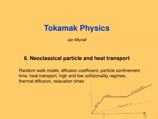
The text book picture of neo-classical diffusion BP contribution decreases in plateau regime and is zero in PS regime: DBP at *=1 is roughly equal to DPS at *=-3/2 Thus, there is a collisionality region with roughly constant D (plateau regime).