Download
1 / 16
160 likes | 300 Vues
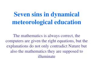
Seven sins in dynamical meteorological education The mathematics is always correct, the computers are given the right equations, but the explanations do not only contradict Nature but also the mathematics they are supposed to illuminate. Seven sins in dynamical meteorological education

E N D
Seven sins in dynamical meteorological education The mathematics is always correct, the computers are given the right equations, but the explanations do not only contradict Nature but also the mathematics they are supposed to illuminate
Seven sins in dynamical meteorological education Professor Richard Reed, Univ. Of Seattle 1988: -Our understanding of the cyclogenesis process has increased tremendously during the last 40 years – at least the computers seem to understand!
3. The Rossby Wave “-I have never understood what a Rossby waves is…” Professor Harold Jeffreys on his deathbed 1987 Lunch discussion at ECMWF 1995: Scientist: -How is the weekend going to be? AP: -Fine, a Rossby wave is seen coming in! Scientist: -But you can’t see Rossby waves??
-Well, Rossby could see them - at least on Christmas Day 1940
Rossby’s wave formula (inspired by Ekman, 1932) C= phase speed, U= zonal flow at 500 hPa, L=wave length, =df/dy c < 0 for large L c >0 for small L
How the Rossby wave was initially misunderstood by Rossby himself
The isobaric channel illustration used by Rossby et al (1939) Only when the paper was published did Rossby realize that he could not use gradient wind balance - it is only applicable on stationary patterns
Jack Bjerknes´ 1937 gradient wind explanation of the progression of waves L Conv Div H H Short waves - the curvature effect dominates
Carl Gustaf Rossby et al (1939) used Bjerknes´ gradient wind idea to illustrate the retrogression of waves High latitude L Div Conv H H Low latitude Long waves - the latitude effect dominates
A very common misunderstanding: This is NOT a Rossby wave! low high f +f==const high low f …but a Constant Absolute Vorticity Trajectory!
There are 5-6 other misleading or erroneous explanations of the Rossby wave before it finally was explained in a kinematically consistent way Rossby (1940), Petterssen (1956), Persson (1993)
Very few seem to have taken notice of a Rossby (1940) correction - and even fewer understood what he meant (Trajectories represented by PV isolines)
Relation between stream lines and trajectories in a progressive flow L H H Larger amplitudes and wave lengths
Relation between stream lines and trajectories in a retrogressive flow L H H Shorter amplitudes and wave lengths
Let us go back to the Constant Absolute Vorticity Trajectory (which is NOT a Rossby wave) +f==const Rossby asked: -Which non-stationary streamlines would correspond to this trajectory?
One and the same CAV trajectory satisfies two types of streamlines (waves) +f==const Short progressive waves Long retrogressive waves