Single Variable Optimization Methods in Chemical Engineering
E N D
Presentation Transcript
Chapter 2Single Variable Optimization Shi-Shang Jang National Tsing-Hua University Chemical Engineering
Contents • Introduction • Examples • Methods of Regional Elimination • Methods of Polynomial Approximation • Methods that requires derivatives • Conclusion
1. Introduction • A single variable problem is such that • Min f(x), x[a,b] • Given f continuous, the optimality criteria is such that: df/dx=0 at x=x* where x* is either a local minimum or a local maximum or a saddle point (a stationary point)
Property of a single variable function (i) a discrete function (ii) a discontinuous function (iii) a continuous function
2. Example • In a chemical plant, the cost of pipes, their fittings, and pumping are important investment cost. Consider a design of a pipeline L feet long that should carry fluid at the rate of Q gpm. The selection of economic pipe diameter D(in.) is based on minimizing the annual cost of pipe, pump, and pumping. Suppose the annual cost of a pipeline with a standard carbon steel pipe and a motor-driven centrifugal pump can be expressed as: Formulate the appropriate single-variable optimization problem for designing a pipe of length 1000ft with a fluid rate of 20gpm. The diameter of the pipe should be between 0.25 to 6 in.
The MATLAB Code for Process Design Example • d=linspace(0.25,6); • l=1000;q=20; • for i=1:100 • hp=4.4e-8*(l*q^3)/d(i)^5 + 1.92e-9*(l*q^2.68) /(d(i)^4.68); • f(i)=0.45*l+0.245*l*d(i)^1.5+3.25*hp^0.5+61.6*hp^0.925+102; • end cost diameter
2. Example- Continued • Carry out a single-variable search of f(x)=3x2+12/x-5 df/dx=6x-12/x2=0
Solutions Methods (1) Analytical Approach • Problem: • Algorithm • Step 1: Set df/dx=0 and solve all stationary points. • Step 2: Select all stationary point x1, x2,…,xNin[a,b]. • Step 3: Compare function values f(x1), f(x2),…,f(xN) and find global minimum.
Example: Polynomial Problem • Example: In the interval of [-2,4]. and f(3)=37, f(-1)=5 3 is the optimum point. f(x) x* x
Example- Inventory Problem • Example : Inventory Control (Economic Order Quantity) • Inventory quantity each time =Q units • Set up cost or ordering cost =$K • Acquisition cost =$C/unit • Storing cost per unit =$h/year • Demand (constant)= units/time unit, this implies ordering period =T=Q/ • Question: What is optimum ordering amount Q?
Solution Objective function =Total cost per year f(Q)=Cost per cycle*
Problems • Cost function must be explicitly expressed • The derivative of the cost function must also be explicitly written down • The derivative equation must be explicitly solved • In many cases, the derivative equation is solved numerically, such as Newton’s method, it is more convenient to solve the optimization problem numerically.
Problems - Continued * x a b Location of global minimum
The Importance of One-dimensional Problem - The Iterative Optimization Procedure • Optimization is basically performed in a fashion of iterative optimization. We give an initial point x0, and a direction s, and then perform the following line search: where * is the optimal point for the objective function and satisfies all the constraints. Then we start from x1 and find the other direction s’, and perform a new line search until the optimum is reached.
The Importance of One-dimensional Problem - The Iterative Optimization Procedure - Continued Consider a objective function Min f(X)= x12+x22, with an initial point X0=(-4,-1) and a direction (1,0), what is the optimum at this direction, i.e. X1=X0 +*(1,0). This is a one -dimensional search for .
The Importance of One-dimensional Problem - The Iterative Optimization Procedure - Continued • The problem can be converted into:
Solution Methods (2) – Numerical Approaches:(i) Numerical Solution to Optimality Condition • Example: Determine the minimum of f(x)=(10x3+3x2+x+5)2 The optimality criteria leads: 2(10x3+3x2+x+5)(30x2+6x+1)=0 Problem: What is the root of the above equation?
Newton’s Method • Consider a equation to be solved: • f(x)=0; • Step 1: give an initial point x0 • Step 2: xn+1=xn-f(xn)/f’(xn) • Step 3: is f(xn) small enough? If not go back to step 2 • Step 4: stop
Newton’s Method (example)MATLAB code x0=10;fx=100;iter=0;ff=[];xx=[]; while abs(fx)>1.e-5 fx=2*(10*x0^3+3*x0^2+x0+5)*(30*x0^2+6*x0+1); ff=[ff;fx]; fxp=2*((30*x0^2+6*x0+1)*(30*x0^2+6*x0+1)+(10*x0^3+3*x0^2+5)*(60*x0+6)); x0=x0-fx/fxp; xx=[xx;x0]; iter=iter+1; end fx = -8.4281e-006 iter = 43 x0 = --0.8599
A Numerical Differentiation Approach • Problem: Find df/dx at a point xk • Approach: • Define xk • Find f(xk) • Find f(xk+ xk ) • Approximate df/dx=[(f(xk+ xk )- f(xk))/ xk ]
A Numerical Differentiation Approach-MATLAB code x0=10;fx=100;iter=0;ff=[];xx=[];dx=0.001; while abs(fx)>1.e-5 fx=2*(10*x0^3+3*x0^2+x0+5)*(30*x0^2+6*x0+1); ff=[ff;fx]; xp=x0+dx; ffp=2*(10*xp^3+3*xp^2+x0+5)*(30*xp^2+6*xp+1); fxp=(ffp-fx)/dx; x0=x0-fx/fxp; xx=[xx;x0]; iter=iter+1; end fx = -2.4021e-006 iter = 25 x0 = -0.8599
Remarks (Numerical Solution to Optimality Condition) • Difficult to formulate the optimality condition • Difficult to solve (multi-solutions, complex number solutions) • Derivative may be very difficult to solve numerically • Function calls are not saved in most cases • New Frontier: Can we simply implement objective function instead of its derivative?
Solution Methods (2) – Numerical Approaches (ii) Reginal Elimination Methods • Theorem: Suppose f is uni-model on the interval a xb, with a minimum at x* (not necessary a stationary point), let x1, x2[a,b] such that a< x1< x2<b, then: • If f(x1)> f(x2) x*[x1,b] • If f(x1)< f(x2) x*[a, x2]
Two Phase Approach • Phase I. Bounding Phase: An initial course search that will bound or bracket the optimum • Phase II. Interval Refinement Phase: A finite sequence of interval reductions or refinements to reduce the initial search interval to desired accuracy.
Phase II- Interval Refinement Phase - Interval Halving • Algorithm • Step 1: Let , L= b-a, find f(xm) • Step 2: Set x1=a+L/4, x2=b-L/4. • Step 3: Find f(x1), if f(x1)<f(xm), then bxm, go to step 1. • if f(x1)>f(xm), continue • Step 4: Find f(x2) • If f(x2)<f(xm), then axm, go to step 1. • If f(x2)>f(xm), then ax1, bx2, go to step 1.
f(x) f2 fm f1 x a x1 xm x2 b Interval Halving
Example:y=(10*x^3+3*x^2+x+5)^2; • global fun_call • a=-3;b=3;l=b-a;xm=(a+b)/2;x1=(a+xm)/2;x2=(xm+b)/2; fm=inter_hal_obj(xm); • iter=1;fun_call=0; • while l>1.e-8 • f1=inter_hal_obj(x1); • if f1<=fm • b=xm;fm=f1; • else • f2=inter_hal_obj(x2); • if f2<=fm • a=xm;fm=f2; • else • a=x1; • b=x2; • end • end • xm=(a+b)/2;x1=(a+xm)/2;x2=(xm+b)/2; %fm=inter_hal_obj(xm); • l=b-a; • iter=iter+1; • end • b =-0.8599 • iter = 31 • fun_call =51
Remarks • At each stage of the algorithm, exactly half of the search is deleted. • At most two function evaluations are necessary at each iteration. • After n iterations, the initial search interval will be reduced to • According to Krefer, the three point search is most efficient among all equal-interval searches.
Phase II- Interval Refinement Phase – The Golden Search (Non-equal Interval Search) • Assume that the total length of the region of search =1, two experiments are done at and 1-. One can compare the above two experiments and hence needs to delete either section between the end point and two trial points. Then one trial point is the new end point, the other is a new comparing point. • Problem: We want the original trial point to be a new trial point, i.e.,. It is possible to solve , =0.61803…
The Algorithm: Golden-Search Method • Step 1: Set L =b-a, =0.61803…, x2=a+L, x1=a+(1-)L • Step 2: Find f(x1), f(x2), compare If f(x1)> f(x2)a=x1, x1x2, go to step 3. If f(x1)< f(x2)b=x2, x2x1, go to step 3. • Step 3: Set L =b-a, x2a+L, if (i) true x1a+(1-)L, if (ii) true. Go to step 2.
MATLAB CODING – The Golden Search • function al_opt=goldsec(op2_func,tol,x0,d) • b=1;a=0;l=b-a; • tau=0.61803;x2=a+tau*l;x1=a+(1-tau)*l; • while l>tol • xx1=x0+x1*d;xx2=x0+x2*d; • y1=feval(op2_func,xx1);y2=feval(op2_func,xx2); • if(y1>=y2) a=x1;x1=x2;l=b-a;x2=a+tau*l; • else • b=x2;x2=x1;l=b-a;x1=a+(1-tau)*l; • end • end • al_opt=b;
Example : The Piping Problem • x0=0.25;d=6-0.25;tol=1.e-6; • al_opt=goldsec('piping',tol,x0,d); • D=x0+al_opt*d; • function y=obj_piping(D) • %D(in) • L=1000;%ft • Q=20;%gpm • hp=4.4e-8*(L*Q^3)/(D^5)+1.92e-9*(L*Q^2.68)/(D^4.68); • y=0.45*L+0.245*L*D^1.5+3.25*(hp)^0.5+61.6*(hp)^0.925+102; • al_opt =0.1000 • D =0.8250 • fun_call =29
Remarks • At each stage, only one function evaluation (or one experiment) is needed. • The length of searching is narrowed by a factor of at each iteration, i.e. • Variable transformation technique may be useful for this algorithm, i.e. set the initial length equal to 1.
Remarks - Continued • Define , N = number of experiments, or function evaluations. • Let E = FR(N)
Solution Methods (2) – Numerical Approaches(iii) Polynomial Approximation Methods –Powell’s Method • Powell’s method is to approximate an objective function by a quadratic function such as f(x)=ax2+bx+c, then it can be shown the optimum is located at x*=-b/2a. • Given the above equation we need to do three experiments (function calls) to fit a quadratic function, let the three experiments (function calls) located at: f(x1), f(x2), f(x3) and let’s rewrite the quadratic equation based on the new notation:
Powell’s Method- Continued • The parameters in the previous slide can be found using three experiments: • At the optimum point, it can be derived based on the above three experiments, such that or
Algorithm (Powell’s Method) • Step 1: Given x0, x, x1=x0+x, , • Step 2: Evaluate f(x0), f(x1) • If f(x1)> f(x0), then x2=x0-x • If f(x1)< f(x0), then x2=x0+2x • Step 3: find f(x2) • Step 4: Find Fmin=min (f(x0), f(x1), f(x2)) • Xmin= x0, x1, x2, such that f(xmin)= Fmin, i=0,1,2. • Step 5: Get a1, a2 • Step 6: Get x*, find f(x*). • Step 7: Check if (i) or (ii) Yes, stop. • No, continue • Step 8: set x2x*, x1xmin, x0one of x0, x1, x2 not xmin • Go to step 4.
Powell’s Method – MATLAB code • function alopt=one_dim_pw(xx,s,op2_func) • dela=0.005; • alp0=0.01; • alpha(1)=alp0;alpha(2)=alpha(1)+dela; • al=alpha(1);x1=xx+al*s; • y(1)=feval(op2_func,x1); • al=alpha(2);x2=xx+s*alpha(2); • y(2)=feval(op2_func,x2); • if(y(2)>=y(1)) alpha(3)=alpha(1)-dela; • else alpha(3)=alpha(1)+2*dela; • end • eps=100; • delta=100; • while eps>0.001|delta>0.001 • x3=xx+s*alpha(3); • y(3)=feval(op2_func,x3); • fmin=min(y);
Powell’s Method – MATLAB code-Continued • if(fmin==y(1)) almin=alpha(1);i=1; • else if(fmin==y(2)) almin=alpha(2);i=2; • else almin=alpha(3);i=3; • end • end • a0=y(1);a1=(y(2)-y(1))/(alpha(2)-alpha(1)); • a2=1/(alpha(3)-alpha(2))*((y(3)-y(1))/(alpha(3)-alpha(1))-(y(2)-y(1))/(alpha(2)-alpha(1))); • alopt=(alpha(2)+alpha(1))/2-a1/(2*a2); • xxopt=xx+alopt*s; • yopt=feval(op2_func,xxopt); • eps=abs(fmin-yopt); • delta=abs(alopt-almin); • for j=1:3 • if(j~=i) alpha(1)=alpha(j); • end • end • alpha(3)=alopt;alpha(2)=almin; • x1=xx+s*alpha(1);x2=xx+s*alpha(2); • y(1)=feval(op2_func,x1);y(2)=feval(op2_func,x2); • end
Example: Piping Design • global fun_call • x0=0.25;x_end=6;l=x_end-x0; • al_opt=one_dim_pw(x0,l,'obj_piping') • D=x0+al_opt*l • fun_call • al_opt = 0.1000 • D =0.8250 • fun_call =61
Comparison – Interval_halving (tol=1.e-6) • l = • 6.8545e-007 • b = • 0.8250 • a = • 0.8250 • iter = • 24 • fun_call = • 63
