Optimization Techniques and Algorithms | Understanding Optimization in Mathematical Modeling
This chapter delves into various optimization methods, including derivative-based and derivative-free algorithms, to enhance decision-making processes. Learn about gradient-based techniques, genetic algorithms, and Simulated Annealing. Understand least squares methods for system identification and the role of optimization algorithms in real-world applications.

Optimization Techniques and Algorithms | Understanding Optimization in Mathematical Modeling
E N D
Presentation Transcript
Chapter 2-OPTIMIZATION G.Anuradha
Contents • Derivative-based Optimization • Descent Methods • The Method of Steepest Descent • Classical Newton’s Method • Step Size Determination • Derivative-free Optimization • Genetic Algorithms • Simulated Annealing • Random Search • Downhill Simplex Search
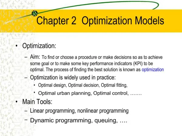
What is Optimization? • Choosing the best element from some set of available alternatives • Solving problems in which one seeks to minimize or maximize a real function
Notation of Optimization Optimize y=f(x1,x2….xn) --------------------------------1 subject to gj(x1,x2…xn) ≤ / ≥ /= bj ----------------------2 where j=1,2,….n Eqn:1 is objective function Eqn:2 a set of constraints imposed on the solution. x1,x2…xn are the set of decision variables Note:- The problem is either to maximize or minimize the value of objective function.
Complicating factors in optimization • Existence of multiple decision variables • Complex nature of the relationships between the decision variables and the associated income • Existence of one or more complex constraints on the decision variables
Types of optimization • Constraint:- Solution is arrived at by maximizing or minimizing the objective function • Unconstraint:- No constraints are imposed on the decision variables and differential calculus can be used to analyze them Examples
Least Square Methods for System Identification • System Identification:- Determining a mathematical model for an unknown system by observing the input-output data pairs • System identification is required • To predict a system behavior • To explain the interactions and relationship between inputs and outputs • To design a controller • System identification • Structure identification • Parameter identification
Structure identification • Apply a priori knowledge about the target system to determine a class of models within which the search for the most suitable model is conducted • y=f(u;θ) y – model’s output u – Input Vector θ – parameter vector
Parameter Identification • Structure of the model is known and optimization techniques are applied to determine the parameter vector θ= θ
Parameter identification • An input ui is applied to both the system and the model • Difference between the target system’s output yi and model’s output yi is used to update a parameter vector θ to minimize the difference • System identification is not a one-pass process; it needs to do both structure and parameter identification repeatedly
Classification of Optimization algorithms • Derivative-based algorithms:- • Derivative-free algorithms
Characteristics of derivative free algorithm • Derivative freeness:- repeated evaluation of objective function • Intuitive guidelines:- concepts are based on nature’s wisdom, such as evolution and thermodynamics • Slower • Flexibility • Randomness:- global optimizers • Analytic Opacity:-knowledge about them are based on empirical studies • Iterative nature:-
Characteristics of derivative free algorithm • Stopping condition of iteration:- let k denote an iteration count and fk denote the best objective function obtained at count k. stopping condition depends on • Computation time • Optimization goal; • Minimal Improvement • Minimal relative improvement
Least Square Estimator • Method of least squares is a standard approach to approximate solution of overdetermined systems. • Least Squares- Overall solution minimizes the sum of the squares of the errors made in solving every single equation • Application—Data Fitting
Types of Least Squares • Least Squares • Linear:- It is a linear combination of parameters. • The model may represent a straight line, a parabola or any other linear combination of functions • Non-Linear:- the parameters appear as functions, such as β2,eβx.If the derivatives are either constant or depend only on the values of the independent variable, the model is linear else non-linear.
Linear model Regression Function
Linear model contd… Using matrix notation Where A is a m*n matrix
Derivative Based Optimization • Deals with gradient-based optimization techniques, capable of determining search directions according to an objective function’s derivative information • Used in optimizing non-linear neuro-fuzzy models, • Steepest descent • Conjugate gradient
1 T T * * ¼ x x x x x x x x x 2 F ( ) = F ( + D ) = F ( ) + Ñ F ( ) D + - - - D Ñ F ( ) D + * * 2 x x x x = = First-Order Optimality Condition For small Dx: If x* is a minimum, this implies: If then But this would imply that x* is not a minimum. Therefore Since this must be true for every Dx,
Second-Order Condition If the first-order condition is satisfied (zero gradient), then A strong minimum will exist at x* if for any Dx°0. Therefore the Hessian matrix must be positive definite. A matrix A is positive definite if: for any z°0. This is a sufficient condition for optimality. A necessary condition is that the Hessian matrix be positive semidefinite. A matrix A is positive semidefinite if: for any z.
Basic Optimization Algorithm or pk - Search Direction ak - Learning Rate
Steepest Descent Choose the next step so that the function decreases: For small changes in x we can approximate F(x): where If we want the function to decrease: We can maximize the decrease by choosing:
Effect of learning rate • More the learning rate the trajectory becomes oscillatory. • This will make the algorithm unstable • The upper limit for learning rates can be set for quadratic functions
Stable Learning Rates (Quadratic) Stability is determined by the eigenvalues of this matrix. Eigenvalues of [I - aA]. (li - eigenvalue of A) Stability Requirement:
Newton’s Method Take the gradient of this second-order approximation and set it equal to zero to find the stationary point:
Conjugate Vectors A set of vectors is mutually conjugate with respect to a positive definite Hessian matrix A if One set of conjugate vectors consists of the eigenvectors of A. (The eigenvectors of symmetric matrices are orthogonal.)
For Quadratic Functions The change in the gradient at iteration k is where The conjugacy conditions can be rewritten This does not require knowledge of the Hessian matrix.
Forming Conjugate Directions Choose the initial search direction as the negative of the gradient. Choose subsequent search directions to be conjugate. where or or
Conjugate Gradient algorithm • The first search direction is the negative of the gradient. • Select the learning rate to minimize along the line. (For quadratic functions.)
Plots Conjugate Gradient Steepest Descent
This is used for finding line minimization methods and their stopping criteria • Initial bracketing • Line searches • Newton’s method • Secant method • Sectioning method

