Optimizing SQL Queries: Techniques and Plans in Database Management
This lecture explores query optimization techniques in SQL, emphasizing System R's optimizer developed at IBM. It covers cost estimation, statistics maintenance, and the significance of left-deep join trees for efficient query execution. Learn about single-relation plans, access paths, and the impact of indexes on query performance. The discussion encompasses operations like selection, projection, aggregation, and the importance of sorting and planning in complex queries with multiple relations, ensuring high efficiency and reduced resource costs.

Optimizing SQL Queries: Techniques and Plans in Database Management
E N D
Presentation Transcript
Query Optimization, part 2 CS634Lecture 13, Mar 24 2014 • Slides based on “Database Management Systems” 3rded, Ramakrishnan and Gehrke
System R Optimizer • Developed at IBM starting in the 1970’s • Most widely used currently; works well for up to 10 joins • Cost estimation • Statistics maintained in system catalogs • Used to estimate cost of operations and result sizes • Query Plan Space • Only the space of left-deep plans is considered • Left-deep plans allow output of each operator to be pipelinedinto the next operator without storing it in a temporary relation • Cartesian products avoided
SQL Query Semantics (pg. 136, 156) • compute the cross product of tables in FROM • delete rows that fail the WHERE clause • project out columns not mentioned in select list or group by or having clauses • group rows by GROUP BY • apply HAVING to the groups, dropping some out • if necessary, apply DISTINCT • if necessary, apply ORDER BY Note this all follows the order of the SELECT clauses, except for projection and DISTINCT, so it’s not hard to remember.
Single-Relation Plans • FROM clause contains single relation • Query is combination of selection, projection, and aggregates (possibly GROUP BY and HAVING, but these come late in the logical progression, so usually less crucial to planning) • Main issue is to select best from all available access paths (either file scan or index) • Access path involves the table and the WHERE clause • Another factor is whether the output must be sorted • E.g., GROUP BY requires sorting • Sorting may be done as separate step, or using an index if an indexed access path is available
Plans Without Indexes • Only access path is file scan • Apply selection and projection to each retrieved tuple • Projection may or may not use duplicate elimination, depending on whether there is a DISTINCT keyword present • GROUP BY: • Write out intermediate relation after selection/projection • Sort intermediate relation to create groups • Apply aggregates on-the-fly per each group • HAVING also performed on-the-fly, no additional I/O needed
Plans With Indexes • There are four cases: • Single-index access path • Each index offers an alternative access path • Choose one with lowest I/O cost • Non-primary conjuncts, projection, aggregates/grouping applied next • Multiple-index access path • Each index used to retrieve set of rids • Rid sets intersected, result sorted by page id • Retrieve each page only once • Non-primary conjuncts, projection, aggregates/grouping applied next
Plans With Indexes (contd.) • Tree-index access path: extra possible use… • If GROUP BY attributes prefix of tree index, retrieve tuples in order required by GROUP BY • Apply selection, projection for each retrieved tuple, then aggregate • Works well for clustered indexes Example: With tree index on rating SELECT count(*), max(age) FROM Sailors S GROUP BY rating
Plans With Indexes (contd.) • Index-only access path • If all attributes in query included in index, then there is no need to access data records: index-only scan • If index matches selection, even better: only part of index examined • Does not matter if index is clustered or not! • If GROUP BY attributes prefix of a tree index, no need to sort! • Example: With tree index on rating • Note count(*) doesn’t require access to row, just RID. SELECT max(rating),count(*) FROM Sailors S
Example Schema • Similar to old schema; rnameadded • Reserves: • 40 bytes long tuple, 100K records, 100 tuples per page, 1000 pages • Sailors: • 50 bytes long tuple, 40K tuples, 80 tuples per page, 500 pages • Assume index entry size 10% of data record size Sailors (sid: integer, sname: string, rating: integer, age: real) Reserves (sid: integer, bid: integer, day: dates, rname: string)
Cost Estimates for Single-Relation Plans • Sequential scan of file: • NPages(R) • Index I on primary key matches selection • Cost is Height(I)+1 for a B+ tree, about 1.2 for hash index • Clustered index I matching one or more selects: • NPages(CI) * product of RF’s of matching selects Quick estimate: Npages(CI) = 1.1*NPages(TableData) i.e. 10% more for needed keys • Non-clustered index I matching one or more selects: • (NPages(I)+NTuples(R)) * product of RF’s of matching selects Quick estimate: Npages(I) = .1*Npages(R) (10% of data size)
Example • File scan: retrieve all 500pages • Clustered Index I on rating (1/NKeys(I)) * (NPages(CI)) = (1/10) * (50+500) pages • UnclusteredIndex I on rating (1/NKeys(I)) * (NPages(I)+NTuples(S)) = (1/10) * (50+40000) pages SELECT S.sid FROM Sailors S WHERE S.rating=8
D D C C D B A C B A B A Queries Over Multiple Relations • In System R only left-deep join treesare considered • In order to restrict the search space • Left-deep trees allow us to generate all fully pipelined plans • Intermediate results not written to temporary files. • Not all left-deep trees are fully pipelined (e.g., sort-merge join) Left-deep
Enumeration of Left-Deep Plans • Among all left-deep plans, we need to determine: • the order of joining relations • the access method for each relation • the join method for each join • Enumeration done in N passes (if N relations are joined): • Pass 1:Find best 1-relation plan for each relation • Pass 2:Find best way to join result of each 1-relation plan (as outer) to another relation - result is the set of all 2-relation plans • Pass N:Find best way to join result of a (N-1)-relation plan (as outer) to the N’th relation - result is the set of all N-relation plans • Speed-up computation using dynamic programming
Enumeration of Left-Deep Plans (contd.) • For each subset of relations, retain only: • Cheapest plan overall, plus • Cheapest plan for each interesting order of the tuples • Interesting order: order that allows execution of GROUP BY without requiring an additional step of sorting, aggregates • Avoid Cartesian products if possible • An N-1 way plan is not combined with an additional relation unless there is a join condition between them • Exception is case when all predicates in WHERE have been used up(i.e., query itself requires a cross-product) • Ex: select … from T1, T2, T3 where T1.x = T2.x • Only one join condition, 3 tables, so end up with cross product
Cost Estimation for Multi-Relation Plans • Two components: • Size of intermediate relations • Maximum tuple count is the product of the cardinalities of relations in the FROMclause • Reduction factor (RF) associated with each condition term • Resultcardinality = Max # tuples * product of all RF’s • Cost of each join operator • Depends on join method
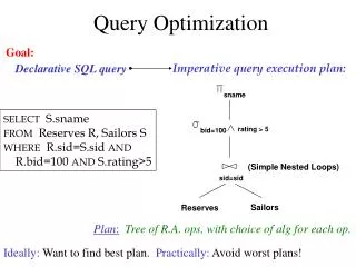
sname rating > 5 bid=100 sid=sid Sailors Reserves Example SELECT S.sname FROM Sailors S, Reserves R WHERE S.sid=R.sid AND S.rating>5 AND R.bid=100 sname sid=sid bid=100 rating > 5 Sailors Reserves
Example Sailors: Unclustered B+ tree on rating Unclustered Hash on sid Reserves: Unclustered B+ tree on bid Pass 1 • Sailors • B+ tree matches rating>5 • Most selective access path • But index unclustered! • Sometimes may prefer scan • Reserves • B+ tree on bid matches selection bid=100 • Cheapest plan
Example Pass 2 • Consider each plan retained from Pass 1 as the outer, and how to join it with the (only) other relation • Sailors outer, Reserves inner • No index matches join condition, this could be done as block nested loop • Reserves outer, Sailors inner • Since we have hash index on sid for Sailors, this could be a cheap plan using an indexed nested loop • Only one matching records, does not matter that index is unclustered • This would mean S.rating>5 is done after join.
Example, cont. • Also need to check sort-merge join • But that requires materialization of input tables, an extra expense • Need to cost all three competing plans, choose least expensive • Note that left-deep plans assume nested-loop joins are in use, so may miss good hash join plans • Note on pg. 500: Oracle considers non-left-deep plans to better utilize hash joins.
Nested Queries • Nested block is optimized independently, with the outer tuple considered as providing a selection condition • Outer block is optimized with the cost of “calling” nested block computation taken into account • Implicit ordering of these blocks means that some good strategies are not considered • The non-nested version of the query is typically optimized better
Nested Queries SELECT S.sname FROM Sailors S WHERE EXISTS (SELECT * FROM Reserves R WHERE R.bid=103 AND R.sid=S.sid) Equivalent non-nested query: SELECTS.sname FROM Sailors S, Reserves R WHERES.sid=R.sid ANDR.bid=103

