Query Optimization

1. Query Optimization Vishy Poosala Bell Labs

2. Outline • Introduction • Necessary Details • Cost Estimation • Result Size Estimation • Standard approach for query optimization • Other ways • Related Concepts

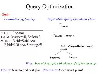
3. Given a query Q, there are several ways (access plans, plans, strategies) to execute Q and find the answer • select z from R,S where R.x=10 and R.y = S.y • selection before join or after or during? What indices to use? • represented as a tree  ⋈ ⋈  S R R S

4. Query optimization is the process of identifying the access plan with the minimum cost • Cost = Time taken to get all the answers • Starting with System-R, most DBMSs use the same algorithm • generate most of the access plans and select the cheapest one • First, how do we determine the cost of a plan? • Then, how long is this process going to take and how do we make it faster?

5. Query execution cost is usually a weighted sum of the I/O cost (# disk accesses) and CPU cost (msec) • w * IO_COST + CPU_COST • Basic Idea: • Cost of an operator depends on input data size, data distribution, physical layout • The optimizer uses statistics about the relations to estimate the cost • Need statistics on base relations and intermediate results ⋈  S R

6. Key parameters • p(R): Relation R’s size in pages • t(R): R’s size in tuples • v(A,R): number of unique values in attribute A • min(A,R), max(A,R): smallest/largest values in attribute A • s(f): A relational operator f’s selectivity factor = ratio of result size over the size of the cross product of the input relations • s(R ⋈S) = t(R ⋈ S)/(t(R)t(S)) • used to estimate t(R ⋈ S)

7. Without Indices • Assume that data is uniformly distributed • Scan • Cost = p(R) • Selection • Cost = p(R) • Result Size • Equality Selection: t(R) / v(A,R) • A > c: t(R) * (max(A,R) - c) / (max(A,R) - min(A,R) • Projection • Cost = p(R) • Size = v(A,R)

8. Join (R ⋈ S) • Tuple Nested Loops (R is outer) • p(R) + t(R) * p(S) • Page Nested Loops • p(R) + p(R) * p(S) • Merge Scan • sort(R) + sort(S) + p(R) + p(S) • sort(R) = 2p(R)* (log (p(R)/w) + 1), w = # buffer pages • Size: t(R) * t(S) / v(A,R) (assuming same number of identical unique values in both relations)

9. With Indices • Cost = Cost(index) + Cost(data) • Parameters for index I • p(I) = size in pages • d(I) = depth of the tree • lp(I) = number of leaf pages • b(I) = # Buckets in hash index

10. Selection • B-tree(primary) = d(I) + p(R) * s • B-tree(secondary) = d(I) + lp(I) * s + s * t(R)/v(A,R) • Hash(primary) = p(R)/b(I) for equality; p(R) for range • Hash(secondary) = p(I)/b(I) + t(R)/v(A,R); p(R) for range • Nested loops (index on inner relation S) • B-tree(primary) = p(R) + (d(I) + p(S)/v(A,S)) * t(R) • B-tree(secondary) = p(R) + (d(I) + lp(I)/v(A,S) + t(S)/v(A,S)) * t(R) • Hash (primary) = p(R) + t(R) * p(S) / b(I) • Hash (secondary) = p(R) + t(R) * (p(I)/b(I) + t(R)/v(A,R) • Merge Join • B-tree(primary) on both = p(R) + p(S) • B-tree(secondary) on R = p(S) + d(I_R) + lp(I_R) + t(R) • Hash: same as no index (sort + store + merge)

11. select z from R,S where R.x=10 and R.y = S.y • selection before join or after or during? • Nested loop join with S as inner • P1: join into temp then select • p(R) + t(R)*p(S) + 2p(R)p(S)/v(y,R) • P2: select into temp then join • p(R) + 2p(R)/v(x,R) + t(R)p(S)/v(x,R) • P3: select while join • p(R) + t(R)p(S)/v(x,R)

12. Lot more options when multiple joins are present • Join is associative: (R ⋈ S) ⋈ T = R ⋈ (S ⋈ T) • In left-deep join trees, the right-hand-side input for each join is a relation, not the result of an intermediate join

13. Consider finding the best join-order for r1r2 . . . rn. • There are (2(n – 1))!/(n – 1)! different join orders for above expression. With n = 7, the number is 665280, with n = 10, thenumber is greater than 176 billion! • No need to generate all the join orders. Using dynamic programming, the least-cost join order for any subset of {r1, r2, . . . rn} is computed only once and stored for future use. • O(n*2^n) (left-deep trees)

14. System-R, Selinger-style, Dynamic Programming(or THE query optimization technique) • A solution consists of an ordered list of the relations to be joined, the join method for each join, and an access plan for the relations (indices) • If the tuples are produced in sorted order on A, the order is interesting if • A participates in another join • or A is an ordered attribute in the SQL query • Idea • Find the best plan for each subset of the relations for each interesting order • Join Heuristics • avoid Cartesian products • use left-deep trees

15. Find the best way to scan each relation for each interesting order and for the unordered case • Find the best way to join each possible pair of relations based on previous step and join heuristics • .. Joins of triples .. • .. • Find best way to join N relations. This is the result • At any point, sub-optimal solutions are removed • expensive out of two same interesting order plans

16. EMP(name, sal, dept); DEPT(dpt, floor, mgr) • select name, mgr from emp, dept where sal >= 30k and floor = 2 and dept.dpt = emp.dpt • EMP has B-tree on sal and on dpt; DEPT has hashing on floor

17. Other Ways • Heuristic-based, Rule-based • Perform most restrictive selection early • Perform all selections before joins • Pick the most “promising” relation to join next (Oracle) • Not guaranteed to give optimal or good solutions • Randomized Algorithms • Iterative Improvement • Simulated Annealing • Not guaranteed, but known to work well

18. Statistics for Size Estimation • Uniform distribution assumption is often invalid • data tends to be skewed • Leads to errors in estimation, sub-optimal plans • Use more realistic statistics • Samples • Histograms: uniform assumption over subsets of data • what subsets do we use? • Equi-depth, equi-width, v-optimal, .. • Polynomials, Wavelets, ... • Have to maintain the statistics as data changes

19. Related Areas • Approximate Query Answering: Answer queries using data summaries, approximately but quickly • E.g., compute avg(salary) within 5% error with 99% confidence in 1/10th of the time • Optimize for fastest first answers • Interactive applications • Parametric Optimization • Keep multiple access plans for different runtime parameters • Optimize for other domains • Image databases, streaming sources, distributed databases • Materialized Views • Store partial results • Maintenance