Query Optimization
Query Optimization. Arash Izadpanah. Introduction: What is Query Optimization?. Query optimization is the process of selecting the most efficient query-evaluation plan from among the many strategies usually possible for processing a given query , especially if the query is complex .

Query Optimization
E N D
Presentation Transcript
Query Optimization ArashIzadpanah
Introduction:What is Query Optimization? Query optimization is the process of selecting the most efficient query-evaluation plan from among the many strategies usually possible for processing a given query, especially if the query is complex.
Introduction:Why Query Optimization is important? • It provides the user with faster results, • It allows the system to service more queries in the same amount of time, • It ultimately reduces the amount of wear on the hardware and allows the server to run more efficiently
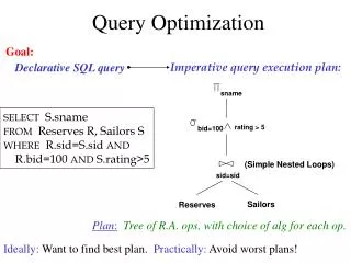
Introduction:Evaluation Plan It defines exactly what algorithm should be used for each operation, and how the execution of the operations should be coordinated.
Introduction:Steps of Cost-Based Query Optimization • Generating expressions that are logically equivalent to the given expression • Annotating the resultant expressions in alternative ways to generate alternative query-evaluation plans • Estimating the cost of each evaluation plan, and choosing the one whose estimated cost is the least These steps interleaved in the query optimizer.
Equivalent (relational-algebra) Expressions Expressions that generate the same set of tuples on every legal database instance • Order of the tuples is irrelevant • Those that generate smaller intermediate relations are preferred.
Equivalence Rules An equivalence rule says that expressions of two forms are equivalent. • The optimizer uses equivalence rules to transform expressions into other logically equivalent expressions.
Equivalence Rules (Continue) • Query optimizers use minimal sets of equivalence rules. • A set of equivalence rules is said to be minimalif no rule can be derived from any combination of the others.
Join Ordering • Reducing the size of temporary results • These expressions are equivalent: (r1 r2) r3 = r1 (r2 r3) • The costs of computing them may differ.
Process of generating equivalent expression • The preceding process is extremely costly both in space and in time
Catalog Information • nr , the number of tuples in the relation r. • br , the number of blocks containing tuples of relation r. • lr , the size of a tuple of relation r in bytes. • fr , the blocking factor of relation r—that is, the number of tuples of relation r that fit into one block.
Catalog Information (Continue) • V (A, r), the number of distinct values that appear in the relation r for attribute A. This value is the same as the size of ∏ A(r). If A is a key for relation r, V (A, r) is nr Every time a relation is modified, we must also update the statistics
Histogram Most databases store the distribution of values for each attribute as a histogram • Values for the attribute are divided into a number of ranges • Histogram associates the number of tuples whose attribute value lies in each range
Selection Size Estimation The size estimate of the result of a selection operation depends on the selection predicate. • Complex selections • Conjunction 1 2. . . n (r) • Disjunction 12. . . n (r) • Negation (r)
Join Size Estimation The Cartesian product r ×s contains nr∗nstuples. Each tuple of r × s occupies lr+ lsbytes, from which we can calculate the size of the Cartesian product. • If R S = , • If R S is a key for R, • If R S in S is a foreign key in S referencing R
Other Operations Estimation • Projection: estimated size of A(r) = V(A,r) • Aggregation : estimated size of AgF(r) = V(A,r) • Set operations • For unions / intersections of selections on the same relation: rewrite and use size estimate for selections • For operations on different relations: • estimated size of r s= size of r + size of s • estimated size of r s = minimum size of r and size of s • estimated size of r – s = r
Other Operations Estimation • Outer join: • Estimated size of r s = size of r s + size of r • Case of right outer join is symmetric • Estimated size of r s = size of r s + size of r + size of s
Estimation of Number of Distinct Values Selections: (r) • If forces A to take a specified value: V(A, (r))=1 • If forces A to take on one of a specified set of values: V(A, (r)) = number of specified values • If the selection condition is of the form Aop r estimated V(A, (r)) = V(A.r) * s • In all the other cases: use approximate estimate of min(V(A,r), n (r) )
Estimation of Number of Distinct Values Joins: r s • If all attributes in A are from restimated V(A, r s) = min (V(A,r), n r s) • If A contains attributes A1 from r and A2 from s, then estimated V(A,rs) = min(V(A1,r)*V(A2 – A1,s), V(A1– A2,r)*V(A2,s),nr s)
Estimation of Number of Distinct Values • Estimation of distinct values are straightforward for projections. • They are the same in A (r) as in r. • The same holds for grouping attributes of aggregation. • For aggregated values • For min(A) and max(A), the number of distinct values can be estimated as min(V(A,r), V(G,r)) where G denotes grouping attributes • For other aggregates, assume all values are distinct, and use V(G,r)
Cost-Based Join Order Selection Choosing the optimal join order for query • Algorithm for finding optimal join orders can can be developed by a dynamic-programming. • reduce execution time • Order of tuples generated by join is also important • It can affect the cost of further joins • Interesting sort order if it could be useful for a later operation
Cost-Based Optimization with Equivalence Rules • Benefit of using equivalence rules is that it is easy to extend the optimizer with new rules to handle different query constructs • Physical equivalence rules allow logical query plan to be converted to physical query plan specifying what algorithms are used for each operation.
Efficient optimizer based on equivalent rules Depends on: • A space efficient representation of expressions which avoids making multiple copies of sub-expressions • Efficient techniques for detecting duplicate derivations of expressions • A form of dynamic programming based on memoization, which stores the best plan for a sub-expression the first time it is optimized, and reuses in on repeated optimization calls on same sub-expression • Cost-based pruning techniques that avoid generating all plans
Heuristics in Optimization Systems may use heuristics to reduce the number of choices that must be made in a cost-based fashion Rules that typically improve execution performance: • Perform selection as early as possible • Perform projection early • Perform most restrictive selection and join operations
Left-deep join orders • Plus heuristics to push selections and projections down the query tree • Reduces optimization complexity and generates plans amenable to pipelined evaluation.
Optimizing Nested Subqueries • Correlation variables are the variables from an outer level query that are used in the nested subquery (these variables are called). • This technique for evaluating a query with a nested subquery is called correlated evaluation.
Optimizing Nested Subqueries • SQL optimizers therefore attempt to transform nested subqueriesinto joins, where possible. • The process of replacing a nested query by a query with a join is called decorrelation.
Materialized Views A view whose contents are computed and stored.
View Maintenance • Task of keeping a materialized view up-to-date with the underlying data is known as materialized view maintenance. • View maintenance can be done by • Manually defining triggers on insert, delete, and update of each relation in the view definition • Manually written code to update the view whenever database relations are updated • Periodic recomputation
Join Operation v= r s • for inserts vnew= vold(irs) • for deletes vnew= vold–(drs)
Selection Operations v = (r) • for inserts vnew= vold(ir) • for deletes vnew= vold - (dr)
Projection Operations A(r) • On insert of a tuple to r, if the resultant tuple is already in A(r) we increment its count, else we add a new tuple with count = 1 • On delete of a tuple from r, we decrement the count of the corresponding tuple in A(r) • If the count becomes 0, we delete the tuple from A(r)
Aggregation Operations count : v = A g count(B)(r) • Whena set of tuples ir is inserted • For each tuple r in ir, if the corresponding group is already present in v, we increment its count, else we add a new tuple with count = 1 • When a set of tuples dr is deleted • for each tuple t in ir.we look for the group t.Ain v, and subtract 1 from the count for the group.
Aggregation Operations sum: v = A g sum(B)(r) • We maintain the sum in a manner similar to count, except we add/subtract the B value instead of adding/subtracting 1 for the count • Additionally we maintain the count in order to detect groups with no tuples. Such groups are deleted from v
Aggregation Operations max: v = A g max(B)(r) • Handling insertions on r is straightforward. • Maintaining the aggregate values min and max on deletions may be more expensive. We have to look at the other tuples of r that are in the same group to find the new minimum
Other Operations v = r s • When a tuple is inserted in r we check if it is present in s, and if so we add it to v. • If the tuple is deleted from r, we delete it from the intersection if it is present.
Handling Expressions Deriving expressions for computing the incremental change to the result of each sub-expressions, starting from the smallest sub-expressions. E1E2 set of tuples to be inserted into E1 is given by D1 tuples to be inserted into E1E2 D1 E2
Query Optimization and Materialized Views • Rewriting queries to use materialized views • it is the job of the query optimizer to recognize when a materialized view can be used to speed up a query. • Replacing a use of a materialized view with the view definition
Materialized View and Index Selection • Materialized view selection: What is the best set of views to materialize? • Index selection: what is the best set of indices to create?
Top-K Optimization select * from r, s where r.B = s.B order by r.A ascending limit 10
Join Minimization • Sometimes more relations are joined than are needed for computation of the query. select r.A, s1.B from r, s as s1, s as s2 where r.B=s1.B and r.B = s2.B and s1.A < 20 and s2.A < 10 • Dropping a relation from a join
Optimization of Updates • Solution 1: Always defer updates • collect the updates and update relation and indices in second pass • Solution 2: Defer only if required • Perform immediate update if update does not affect attributes in where clause, and deferred updates otherwise.
Multiquery Optimization and Shared Scans • Multiquery Optimization : • Complex queries may in fact have subexpressionsrepeated in different parts of the query • It can be similarly exploited, to reduce query evaluation cost • Shared-scan: • Instead of reading the relation repeatedly from disk, • data are read once from disk, and pipelined to each of the queries
Parametric Query Optimization select * from r natural join s where r.a < $1 • Parametric Query Optimization: • optimizer generates a set of plans, optimal for different values of $1

