Query Optimization
This document explores advanced query optimization strategies, focusing on size estimation, join ordering, and predicate pushdown. It covers schema designs for Products and Sales tables and provides transformation rules that guide effective query rewriting. Discussions include optimizing group by and join operations, improving selection predicates, and utilizing histograms for accurate size estimations. Additionally, the document emphasizes minimizing the size of intermediate joins and encourages creativity in query rewriting. Ideal for database professionals seeking to maximize query performance.

Query Optimization
E N D
Presentation Transcript
Query Optimization May 31st, 2002
Today • A few last transformations • Size estimation • Join ordering • Summary of optimization
Rewrites: Group By and Join • Schema: • Product (pid, unitprice,…) • Sales(tid, date, store, pid, units) • Trees: Join groupBy(pid) Sum(units) groupBy(pid) Sum(units) Join Products Filter (in NW) Products Filter (in NW) Scan(Sales) Filter(date in Q2,2000) Scan(Sales) Filter(date in Q2,2000)
Rewrites:Operation Introduction groupBy(cid) Sum(amount) • Schema: (pid determines cid) • Category (pid, cid, details) • Sales(tid, date, store, pid, amount) • Trees: Join groupBy(cid) Sum(amount) groupBy(pid) Sum(amount) Join Category Filter (…) Category Filter (…) Scan(Sales) Filter(store IN {CA,WA}) Scan(Sales) Filter(store IN {CA,WA})
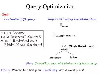
sname sid=sid (Scan; (Scan; write to write to rating > 5 bid=100 temp T2) temp T1) Reserves Sailors sname rating > 5 bid=100 sid=sid Sailors Reserves Query Rewriting: Predicate Pushdown The earlier we process selections, less tuples we need to manipulate higher up in the tree. Disadvantages?
Query Rewrites: Predicate Pushdown (through grouping) Select bid, Max(age) From Reserves R, Sailors S Where R.sid=S.sid GroupBy bid Having Max(age) > 40 Select bid, Max(age) From Reserves R, Sailors S Where R.sid=S.sid and S.age > 40 GroupBy bid • For each boat, find the maximal age of sailors who’ve reserved it. • Advantage: the size of the join will be smaller. • Requires transformation rules specific to the grouping/aggregation • operators. • Will it work work if we replace Max by Min?
Query Rewrite:Predicate Movearound Sailing wiz dates: when did the youngest of each sailor level rent boats? Select sid, date From V1, V2 Where V1.rating = V2.rating and V1.age = V2.age Create View V1 AS Select rating, Min(age) From Sailors S Where S.age < 20 Group By rating Create View V2 AS Select sid, rating, age, date From Sailors S, Reserves R Where R.sid=S.sid
Query Rewrite: Predicate Movearound Sailing wiz dates: when did the youngest of each sailor level rent boats? Select sid, date From V1, V2 Where V1.rating = V2.rating and V1.age = V2.age, age < 20 First, move predicates up the tree. Create View V1 AS Select rating, Min(age) From Sailors S Where S.age < 20 Group By rating Create View V2 AS Select sid, rating, age, date From Sailors S, Reserves R Where R.sid=S.sid
Query Rewrite: Predicate Movearound Sailing wiz dates: when did the youngest of each sailor level rent boats? Select sid, date From V1, V2 Where V1.rating = V2.rating and V1.age = V2.age, andage < 20 First, move predicates up the tree. Then, move them down. Create View V1 AS Select rating, Min(age) From Sailors S Where S.age < 20 Group By rating Create View V2 AS Select sid, rating, age, date From Sailors S, Reserves R Where R.sid=S.sid, and S.age < 20.
Query Rewrite Summary • The optimizer can use any semantically correct rule to transform one query to another. • Rules try to: • move constraints between blocks (because each will be optimized separately) • Unnest blocks • Especially important in decision support applications where queries are very complex. • In a few minutes of thought, you’ll come up with your own rewrite. Some query, somewhere, will benefit from it. • Theorems?
Size Estimation and Reduction Factors SELECT attribute list FROM relation list WHEREterm1AND ... ANDtermk • Consider a query block: • Maximum # tuples in result is the product of the cardinalities of relations in the FROM clause. • Reduction factor (RF) associated with eachtermreflects the impact of the term in reducing result size. Resultcardinality = Max # tuples * product of all RF’s. • Implicit assumption that terms are independent! • Term col=value has RF 1/NKeys(I), given index I on col • Term col1=col2 has RF 1/MAX(NKeys(I1), NKeys(I2)) • Term col>value has RF (High(I)-value)/(High(I)-Low(I))
Histograms • Key to obtaining good cost and size estimates. • Come in several flavors: • Equi-depth • Equi-width • Which is better? • Compressed histograms: special treatment of frequent values.
Histograms Employee(ssn, name, salary, phone) • Maintain a histogram on salary: • T(Employee) = 25000, but now we know the distribution
Plans for Single-Relation Queries(Prep for Join ordering) • Task: create a query execution plan for a single Select-project-group-by block. • Key idea: consider each possible access path to the relevant tuples of the relation. Choose the cheapest one. • The different operations are essentially carried out together (e.g., if an index is used for a selection, projection is done for each retrieved tuple, and the resulting tuples are pipelined into the aggregate computation).
SELECT S.sid FROM Sailors S WHERE S.rating=8 Example • If we have an Index on rating: • (1/NKeys(I)) * NTuples(R) = (1/10) * 40000 tuples retrieved. • Clustered index: (1/NKeys(I)) * (NPages(I)+NPages(R)) = (1/10) * (50+500) pages are retrieved (= 55). • Unclustered index: (1/NKeys(I)) * (NPages(I)+NTuples(R)) = (1/10) * (50+40000) pages are retrieved. • If we have an index on sid: • Would have to retrieve all tuples/pages. With a clustered index, the cost is 50+500. • Doing a file scan: we retrieve all file pages (500).
Determining Join Ordering • R1 R2 …. Rn • Join tree: • A join tree represents a plan. An optimizer needs to inspect many (all ?) join trees R3 R1 R2 R4
Types of Join Trees • Left deep: R4 R2 R5 R3 R1
Types of Join Trees • Bushy: R3 R2 R4 R5 R1
Types of Join Trees • Right deep: R3 R1 R5 R2 R4
Problem • Given: a query R1 R2 … Rn • Assume we have a function cost() that gives us the cost of every join tree • Find the best join tree for the query
Dynamic Programming • Idea: for each subset of {R1, …, Rn}, compute the best plan for that subset • In increasing order of set cardinality: • Step 1: for {R1}, {R2}, …, {Rn} • Step 2: for {R1,R2}, {R1,R3}, …, {Rn-1, Rn} • … • Step n: for {R1, …, Rn} • A subset of {R1, …, Rn} is also called a subquery
Dynamic Programming • For each subquery Q ⊆ {R1, …, Rn} compute the following: • Size(Q) • A best plan for Q: Plan(Q) • The cost of that plan: Cost(Q)
Dynamic Programming • Step 1: For each {Ri} do: • Size({Ri}) = B(Ri) • Plan({Ri}) = Ri • Cost({Ri}) = (cost of scanning Ri)
Dynamic Programming • Step i: For each Q ⊆ {R1, …, Rn} of cardinality i do: • Compute Size(Q) (later…) • For every pair of subqueries Q’, Q’’ s.t. Q = Q’ U Q’’compute cost(Plan(Q’) Plan(Q’’)) • Cost(Q) = the smallest such cost • Plan(Q) = the corresponding plan
Dynamic Programming • Return Plan({R1, …, Rn})
Query Optimization Summary • Parse query, represent as multiple blocks. • Use transformations: merge blocks, move predicates among blocks. • Compute a join order for every block. Push selections and projections. • Create a scheduling for the block plans, and the schedule the different blocks. • This is one way to do things. There are others.

