Chapter 2 Deterministic Optimization Models in Operations Research
Chapter 2 Deterministic Optimization Models in Operations Research. EXAMPLE 2.1: Two Crude Petroleum.

Chapter 2 Deterministic Optimization Models in Operations Research
E N D
Presentation Transcript
Chapter 2Deterministic Optimization Models in Operations Research
EXAMPLE 2.1: Two Crude Petroleum Two Crude Petroleum runs a small refinery on the Texas coast. The refinery distills crude petroleum from two sources, Saudi Arabia and Venezuela, into the three main products: gasoline, jet fuel and lubricants. The two crudes differ in chemical composition and yield different product mixes. Each barrel of Saudi crude yields 0.3 barrel of gasoline, 0.4 barrel of jet fuel, and 0.2 barrel of lubricants. Each barrel of Venezuelan crude yields 0.4 barrel of gasoline, 0.2 barrel of jet fuel and 0.3 barrel of lubricants. The remaining 10% is lost to refining.
EXAMPLE 2.1: Two Crude Petroleum The crudes differ in cost and availability. Two Crude can purchase up to 9000 barrels per day from Saudi Arabia at $20 per barrel. Up to 6000 barrels per day of Venezuelan petroleum are available at the lower cost of $15 per barrel. Two contracts require it to produce 2000 barrels per day of gasoline,1500 barrels per day of jet fuel and 500 barrels per day of lubricants. How can these requirements be fulfilled most efficiently?
2.1 Decision Variables, Constraints, and Objective Functions • Decision Variables: Variables in optimization models represent the decisions to be taken. [2.1] • Input parameters: fixed information • Yields, Cost, Availability, Requirements • Decision Variables: x1barrels of Saudi crude refined /day (in 1000s) x2barrels of Venezuelan crude refined /day (in 1000s) (2.1)
Constraints • Variable-type Constraints specify the domain of definition for decision variables: the set of values for which the variables have meaning. [2.2] Nonnegativity: x1,x2 0 (2.2)
Constraints • Main Constraints of optimization models specify the restrictions and interactions, other than variable-type, that limit decision variable values. [2.3] 0.3 x1 + 0.4 x2 2.0 (gasoline) 0.4 x1 + 0.2 x2 1.5 (jet fuel) 0.2 x1 + 0.3 x2 0.5 (lubricants) x1 9 (Saudi) x2 6 (Venezuelan) (2.3) (2.4)
Objective Functions • Objective Functions in optimization models quantity the decision consequences to be maximized or minimized. [2.4] min 20 x1 + 15 x2 (2.5)
Standard Model The standard statement of an optimization model has the form max or min (objective function(s)) s.t. (main constraints) (variable-type constraints) • min 20 x1 + 15 x2 (total cost) s.t. [2.5] 0.3 x1 + 0.4 x2 2.0 (gasoline) 0.4 x1 + 0.2 x2 1.5 (jet fuel) 0.2 x1 + 0.3 x2 0.5 (lubricants) (2.6) x1 9 (Saudi) x2 6 (Venezuelan) x1,x2 0 (nonnegativity)
2.2 Graphic Solution and Optimization Outcomes • Graphic solution solves 2 and 3-variable optimization models by plotting elements of the model in a coordinate system corresponding to the decision variables. • Feasible set (or region) of an optimization model is the collection of choices for decision variables satisfying all model constraints. [2.6] • Graphic solution begins with a plot of the choices for the decision variables that satisfy variable-type constraints.
Feasible Set (Region)Variable-type Constraints x2 8 7 6 5 4 3 2 1 1 2 3 4 5 6 7 8 9 10 x1
Feasible Set (Region)Main Constraints • The set of points satisfying an equality constraint plots as a line or curve. [2.8] • The set of points satisfying an inequality constraint plots as a boundary line or curve, where the constraint holds with equality, together with all points on whichever side of the boundary satisfy the constraint as an inequality. [2.9]
Feasible Set (Region)Main Constraints x2 8 7 6 5 4 0.3x1+0.4x2 2 3 2 1 1 2 3 4 5 6 7 8 9 10 x1
Feasible Set (Region)Main Constraints • The feasible set (or region) for an optimization model is plotted by introducing constraints one by one, keeping track of the region satisfying all at the same time. [2.10]
Feasible Set (Region)Variable-type Constraints x2 8 7 6 x2 6 5 x1 9 4 3 0.3x1+0.4x2 2 0.4x1+0.2x2 1.5 2 0.2x1+0.3x2 0.5 1 1 2 3 4 5 6 7 8 9 10 x1
Objective Functions c(x1, x2) 20x1+15x2 • Objective functions are normally plotted in the same coordinate system as the feasible set of an optimization model by introducing contours – lines or curves through points having equal objective function value. [2.11] (2.8)
Objective Functions x2 8 20x1+15x2 7 6 5 4 120 3 90 2 60 1 1 2 3 4 5 6 7 8 9 10 x1
Optimal Solutions • An optimal solution is a feasible choice for decision variables with objective function value at least equal to that of any other solution satisfying all constraints. [2.12] • Optimal solutions show graphically as points lying on the best objective function contour that intersects the feasible region. [2.13]
Optimal Solutions x2 8 7 6 x2 6 5 x1 9 4 3 0.3x1+0.4x2 2 0.4x1+0.2x2 1.5 2 0.2x1+0.3x2 0.5 1 1 2 3 4 5 6 7 8 9 10 x1
Optimal Values • An optimal value in an optimization model is the objective function value of any optimal solutions. [2.14] • An optimization model can have only one optimal value. [2.15]
Unique versus Alternative Optimal Solutions • An optimization model may have a unique optimal solution orseveral alternative optimal solutions. [2.16] • Unique optimal solutions show graphically by the optimal-value contour intersecting the feasible set at exactly one point. If the optimal-value contour intersects at more than one point, the model has alternative optimal solutions. [2.17]
Alternative Optimal Solutions x2 8 20x1+10x2 7 6 x2 6 5 x1 9 4 3 0.3x1+0.4x2 2 0.4x1+0.2x2 1.5 2 0.2x1+0.3x2 0.5 1 1 2 3 4 5 6 7 8 9 10 x1
Infeasible Models • An optimization model is infeasible if no choice of decision variables satisfies all constraints. [2.18] • An infeasible model shows graphically by no point fallingwithin the feasibleregion for all constraints. [2.19]
Infeasible Models x2 8 7 x1 2 6 5 4 3 x2 2 0.3x1+0.4x2 2 0.4x1+0.2x2 1.5 2 0.2x1+0.3x2 0.5 1 1 2 3 4 5 6 7 8 9 10 x1
Unbounded Models • An optimization model is unbounded when feasible choices of the decision variables can produce arbitrarily good objective function values.[2.20] • Unboundedmodels show graphically by therebeing points in the feasible set lying on ever-better objective function contours. [2.21]
Unbounded Models x2 8 -2x1+15x2 7 6 x2 6 5 4 3 0.3x1+0.4x2 2 0.4x1+0.2x2 1.5 2 0.2x1+0.3x2 0.5 1 1 2 3 4 5 6 7 8 9 10 x1
2.3 Large-scale Optimization Models and Indexing • Indexing or subscripts permit representing collections of similar quantities with a single symbol.
EXAMPLE 2.2: Pi Hybrids Pi Hybrid, a large manufacturer of corn seed, operates l=20 facilities producing seeds of m=25 hybrid corn varieties and distributes them to customers in n=30 sales regions. They want to know how to carry out these production and distribution operations at minimum cost. Parameters: • Cost per bag of producing each hybrid at each facility • Corn processing capacity of each facility in bushels • Number of bushels of corn must be processed • Demand (bags) of each hybrid in each region • Cost of shipping (per bag) from facility to region
Indexing • The first step in formulating a large optimization model is to choose appropriate indexes for the different dimensions of the problem. [2.22] f production facility number (f = 1, …, l) h hybrid variety number (h = 1,…, m) r sales region number (r = 1, …, n)
Indexing Decision Variables • It is usually appropriate to use separate indexes for each problem dimension over which a decision variable or input parameter is defined. [2.23] xf,h number of bags of hybrid h produced at facility f (f = 1, …, l; h = 1,…, m) yf,h,r number of bags of hybrid h shipped from facility f to sales region r (f=1, …, l; h=1,…, m; r=1, …, n)
Indexing Input Parameters • To describe large-scale optimization models, it is usually necessary to assign indexed symbolic names to most input parameters, even though they are being treated as constant. [2.24] pf,h cost per bag of producing hybrid h at facility f uf corn processing capacity (in bushels) of facility f ah number of bushels of corn must ne processed for a bag of hybrid h dh,r demand of hybrid h in sales region r sf,h,r cost per bag of of shipping hybrid h from facility f to sales region r
Objective Function • Total cost = total production cost + total shipping cost
Indexing Families of Constraints • Families of similar constraints distinguished by indexes may be expressed in a single-line format (constraint for fixed indexes) (ranges of indexes) Which implies one constraint for each combination of indexes in the ranges specified. [2.25]
Pi Hybrids Example Model s.t. ; ; ; ; ; (2.10)
How Models Become Large • Optimization models become large mainly by relatively small number of objective function and constraint elements being repeated many times for different periods, locations, products, and so on. [2.26]
2.4 Linear and Nonlinear Programs The general form of a mathematical program or (single objective) optimization model is min or max f(x1, …, xn) subject to: ,… Where f, g1,…,gmare given functions of decision variables x1,…,xn, and b1, …, bmare specified constant parameters. [2.27]
Two Crude Petroleum f(x1, x2) 20 x1 + 15 x2 g1(x1, x2) 0.3 x1 + 0.4 x2 g2(x1, x2) 0.4 x1 + 0.2 x2 g3(x1, x2) 0.2 x1 + 0.3 x2 g4(x1, x2) x1 g5(x1, x2) x2 g6(x1, x2) x1 g7(x1, x2) x2 RHSs: b1 = 2.0, b2= 1.5, b3= 0.5, b4= 9, b5= 6, b6 = 0, b7= 0 min 20 x1 + 15 x2 s.t. 0.3 x1 + 0.4 x2 2.0 0.4 x1 + 0.2 x2 1.5 0.2 x1 + 0.3 x2 0.5 x1 9 x2 6 x1,x2 0 (2.11)
Linear Functions A function is linear if it is a constant-weighted sum of decision variables. Otherwise, it is nonlinear. [2.28]
Linear and Nonlinear Programs Defined • An optimization model in functional form [2.27] is a linear program (LP) if the (single) objective function f and all constraint functions g1, …, gmare linear in the decision variables. Also, decision variables should be able to take on whole-number or fractional values. [2.29] • An optimization model in functional form [2.27] is a nonlinear program (NLP) if the (single) objective function for any of the constraint functions g1, …, gmis nonlinear in the decision variables. Also, decision variables should be able to take on whole-number or fractional values. [2.30]
Example 2.3: E-mart E-mart, a large European variety store, sells products in m=12 major merchandise groups, such as children’s wear, candy, music, toys, and electric. Advertising is organized into n=15 campaign formats promoting specific merchandise groups through a particular medium (catalog, press, or television). For example, one variety of campaign advertises children’s wear in catalogs, another promotes the same product line in newspapers and magazines, while a third sells toys with television. The profit margin (fraction) for each merchandise group is known, and E-mart wishes to maximize the profit gained from allocating its limited advertising budget across the campaign alternatives.
Indexing, Parameters, and Decision Variables for E-mart • Indexing gmerchandise group number (g = 1, …, m) ccampaign type number (c = 1, …, n) • Input parameters pg profit, as a fraction of sales, realized from merchandise group g b available advertising budget • Decision variables xc amount spent on campaign type c
Nonlinear Response • When there is an option, linear constraint and objective functions are preferred to nonlinear ones in optimization models because each nonlinearity of an optimization model usually reduces its tractability as compared to linear forms. [2.31] • Linear functions implicitly assume that each unit increase in a decision variable has the same effect as the preceding increase: equal returns to scale. [2.32] (sales increase in group g due to campaign c) = sg,clog (xc+1) where sg,c parameter relating advertising expenditure in campaign c to sales growth in merchandise group g (2.12)
E-mart Model s.t. (2.13)
2.5 Discrete or Integer Programs • Discrete optimization models include decisions of a logical character qualitatively different from those of linear or nonlinear programs. • Discrete optimization models are also called integer programs, mixed-integer programs, and combinatorial optimization problems.
Example 2.4: Bethlehem Ingot Mold Bethlehem Steel Corporation needs to choose ingot sizes and molds. In their process for making steel products, molten output from main furnaces is poured into large molds to produce rectangular blocks called ingots. After the molds have been removed, the ingots are reheated and rolled into product shapes such as l-beams and flat sheets. Bethlehem’s mills using this process make approximately n = 130 different products. The dimensions of ingots directly affect efficiency. For example. ingots of one dimension may be easiest to roll into l-beams, but another produces sheet steel with less waste. Some ingot sizes cannot be used at all in making certain products. A careful examination of the best mold dimensions for different products yielded m = 600 candidate designs. However, it is impractical to use more than a few because of the cost of handling and storage. We wish to select at most p= 6 and to minimize the waste associated with using them to produce all n products.
Indexing and Parameters of the Bethlehem Example • Indexing imold design number (i = 1, …, m) j product number (j = 1, …, n) • Input parameters ci,jamount of waste caused by using mold i on product j Ijcollection of indexes i corresponding to molds that could be used for product j . IfiIj, mold i is feasible for product j
Discrete versus Continuous Decision Variables • A variable is discrete if it is limited to a fixed or countable set of values. Often, the choices are only 0 and 1. [2.33] • Decision variables yi xi,j
Discrete versus Continuous Decision Variables • A variable is continuous if it can take any value in a specified interval. [2.34] • When there is an option, such as when optimal variable magnitudes are likely to be large enough that fractions have no practical importance, modeling with continuous variables is preferred to discrete because optimizations over continuous variables are generally more tractable than are ones over discrete variables. [2.35]
Bethlehem Ingot Mold ExampleModel s.t. (2.14)