Query Optimization: Choosing the Best Execution Plan
Understand query optimization process, generate equivalent expressions, estimate costs, and choose the optimal evaluation plan for efficient database querying. Learn about relational expressions and equivalence rules in data management.

Query Optimization: Choosing the Best Execution Plan
E N D
Presentation Transcript
Chapter 13: Query Optimization Data Management for Big Data 2018-2019 (spring semester) Dario Della Monica These slides are a modified version of the slides provided with the book The originalversion of the slidesisavailable at: https://www.db-book.com/
Chapter 13: Query Optimization • Introduction • Generating Equivalent Expressions • Statistical Information for Cost Estimation (the Catalog) • Choice of Evaluation Plans • Dynamic Programming for Choosing Evaluation Plans
Introduction • Query optimization is the process the best query execution plan (QEP) among the many possible ones • Alternative ways to execute a given query • Equivalent relational algebra expressions • Different implementation choices for each relational algebra operation INSTR(i_id, name, dept_name, ...) COURSE(c_id, title, ...) TEACHES(i_id, c_id, ...) The name of all instructors in the department of Music together with the titles of all courses they teach SELECT I.name, C.title FROM INSTR I, COURSE C, TEACHES T WHERE I.i_id = T.i_id AND T.c_id = C.c_id AND dept_name=“Music”
Introduction (Cont.) • A query evaluation plan (QEP) defines exactly what algorithm is used for each operation, and how the execution of the operations is coordinated • Find out how to view query execution plans on your favorite database
Introduction (Cont.) • Cost difference between query evaluation plans can be enormous • E.g. seconds vs. days in some cases • Steps in cost-based query optimization • Generate logically equivalent expressions using equivalence rules • Annotate resulting expressions to get alternative QEP • Evaluate/estimate the cost (execution time) of each QEP • Choose the cheapest QEP based on estimated cost • Estimation of QEP cost based on: • Statistical information about relations (stored in the Catalog) • number of tuples, number of distinct values for an attribute • Statistics estimation for intermediate results • to compute cost of complex expressions • Cost formulae for algorithms, computed using statistics
Transformation of Relational Expressions • Two relational algebra expressions are said to be equivalent if the two expressions generate the same set of tuples on every legal database instance • Note: order of tuples is irrelevant (and also order of attributes) • we don’t care if they generate different results on databases that violate integrity constraints (e.g., uniqueness of keys) • In SQL, inputs and outputs are multisets of tuples • Two expressions in the multiset version of the relational algebra are said to be equivalent if the two expressions generate the same multiset of tuples on every legal database instance • We focus on relational algebra and treat relations as sets • An equivalence rule states that expressions of two forms are equivalent • One can replace an expression of first form by one of the second form, or vice versa
Equivalence Rules 1. Conjunctive selection operations can be deconstructed into a sequence of individual selections. 2. Selection operations are commutative. • Only the last in a sequence of projection operations is needed, the others can be omittedwhere • Selections can be combined with Cartesian products and theta joins. • (E1X E2) = E1 E2 • 1(E12 E2) = E11 2E2
Equivalence Rules (Cont.) 5. Theta-join (and thus natural joins) operations are commutative.E1 E2 = E2E1 (but the order is important for efficiency) 6. (a) Natural join operations are associative: (E1 E2) E3 = E1 (E2 E3) (again, the order is important for efficiency) (b) Theta joins are associative in the following manner: (E1 1E2) 23E3 = E1 1 3 (E22 E3) where 1involves attributes from only E1 and E2and 2involves attributes from only E2 and E3 More equivalences at Ch. 13.2 of the book⋆ ⋆ Silberschatz, Korth, and Sudarshan, Database System Concepts, 6° ed.
Exercise ( R S ) T = R ( S T ) Definition (left outer join): the result of a left outer join T = R S is a super-set of the result of the join T’ = R S in that all tuples in T’ appear in T. In addition, T preserve those tuples that are lost in the join, by creating tuples in T that are filled with null values STUDstud_id name surname 1 gino bianchi 2 filippo neri 3 mario rossi STUD TAKES stud_idnamesurnamecoursegrade 1 gino bianchi Math 30 1 gino bianchi Algebra 26 2 filippo neri Progr. 22 2 filippo neri Math 28 2 filippo neri Logic 30 3 mario rossi nullnull TAKESstud_id course grade 1 Math 30 1 Algebra 26 2 Progr. 22 2 Math 28 2 Logic 30 ⋆ Silberschatz, Korth, and Sudarshan, Database System Concepts, 6° ed. Create equivalence rules to push selection inside a left outer join Ex. 13.1(c) ⋆ Disprove the equivalence Ex. 13.1(d) ⋆
Solutions • Create equivalence rules involving left outer join and selection ( R S ) = ( R ) S where uses only attributes of R • Disprove the equivalence ( R S ) T = R ( S T ) S R T S T R S R ( S T ) ( R S ) T
Solutions (cont’d) • Disprove the equivalence ( R S ) T = R ( S T ) Another counter-example (to fix for solution given on the webpage of the book) S R T S T R S ( R S ) T R ( S T )
Enumeration of Equivalent Expressions • Query optimizers use equivalence rules to systematically generate expressions equivalent to the given expression • Can generate all equivalent expressions as follows: • Repeat • apply all applicable equivalence rules on every sub-expression of every equivalent expression found so far • add newly generated expressions to the set of equivalent expressions Until no new equivalent expressions are generated above • The above approach is very expensive in space and time • Space: sharing (re-using) common sub-expressions(detect duplicate sub-expressions and share one copy) • Time: • Dynamic programming • Greedy techniques (select best choices at each step) • Heuristics, e.g., single-relation operations(selections, projections) are pushed inside (performed earlier) E1 E2
Cost Estimation • Cost of each operator computed as described in Chapter 12 ⋆ • Need statistics of input relations • E.g. number of tuples, sizes of tuples • Inputs can be results of sub-expressions • Need to estimate statistics of expression results • E.g., selectivity rate based on number of distinct values for an attribute • Statistics are collected in the Catalog ⋆ Silberschatz, Korth, and Sudarshan, Database System Concepts, 6° ed.
Statistical Information for Cost Estimation • Statistics information for cost estimation is maintained in the Catalog • The catalog is itself stored in the database • It contains: • nr: number of tuples in a relation r • br: number of blocks containing tuples of r • lr: size of a tuple of r (in bytes) • fr: blocking factor of r — i.e., the number of tuples of r that fit into one block • V(A, r): number of distinct values that appear in r for attribute A; same as the size of A(r) • min(A,r): smallest value appearing in relation r for attribute A; • max(A,r): largest value appearing in relation r for attribute A; • If tuples of r are stored together physically in a file, then:
Histograms • Histogram on attribute age of relation person • For each range • Number of records (tuples) with value in the range • Also, number of distinct values in the range • Without histogram information, uniform distribution is assumed
Selection Size Estimation • A=v(r ) • nr / V(A,r) : number of records that will satisfy the selection (uniform distribution) • Equality condition on a key attribute: size estimate = 1 • A v(r ) (case of A V(r) is symmetric) • n: estimated number of tuples satisfying the condition is computed assuming that min(A,r) and max(A,r) are available in catalog • n = 0 if v < min(A,r) • n = otherwise (uniform distribution) • In absence of statistical information or when v is unknown at time of cost estimation (e.g., v is computed at run-time by the application using the DB) n is assumed to benr / 2 • If histograms are available, we can refine above estimate by using values for restricted ranges instead of values referring to the entire domain (nr , V(A,r), min(A, r), max(A, r) )
Choice of Evaluation Plans • Must consider the interaction of evaluation techniques when choosing evaluation plans • choosing the cheapest algorithm for each operation independently may not yield best overall algorithm. E.g. • merge-join may be costlier than hash-join, but may provide a sorted output which reduces the cost for an outer level aggregation • nested-loop join may provide opportunity for pipelining • Practical query optimizers incorporate elements of the following two broad approaches: 1. Search all the plans and choose the best plan in a cost-based fashion 2. Uses heuristics to choose a plan
Cost-Based Optimization • Consider finding the best join-order for r1r2 . . . rn. • There are (2(n – 1))!/(n – 1)! different join orders for above expression. With n = 7, the number is 665280, with n = 10, thenumber is greater than 17.6 billion! • No need to generate all the join orders. Exploiting some monotonicity (optimal substructure property), the least-cost join order for any subset of {r1, r2, . . ., rn} is computed only once.
Cost-Based Optimization: An example • Consider finding the best join-order for r1r2 r3r4r5 • Number of possible different join orderings: • The least-cost join order for any subset of { r1, r2, r3, r4, r5 } is computed only once • Assume we want to compute N123/45 : number of possible different join orderings where r1, r2, r3 sare grouped together, e.g., (r2r3 r1)(r5r4 ) r4(r5 (r1(r2 r3))) (r1r2 r3)r4r5 • The naïve approach • N123/45 = N123 * N45 • N123 = (N123 : # ways of arranging r1, r2, and r3) • N45 = N123 = 12 (N45 : # ways of arranging r4 and r5 wrt. block of r1, r2, and r3) • N123/45 = 12 * 12 = 144 • Exploiting optimal substructure property: • compute only once best ordering for r1r2 r3 : 12 possibilities (N123) • compute best ordering for R123r4 r5 : 12 possibilities (N45) • Therefore, N123/45 = 12 + 12 = 24
Dynamic Programming in Optimization • To find best join tree (equivalently, best join order) for a set of n relations: • To find best plan for a set S of n relations, consider all possible plans of the form: S’ (S \ S’ ) for every non-empty subset S’ of S • Recursively compute costs of best join orders for subsets S’ and S \ S’ to find the cost of each plan. Choose the cheapest of the 2n– 2 alternatives • Base case for recursion: single relation access plan • Apply all selections on Ri using best choice of indices on Ri • When a plan for a subset is computed, store it and reuse it when it is required again, instead of re-computing it • Dynamic programming
Join Order Optimization Algorithm procedure findbestplan(S)if (bestplan[S].cost )return bestplan[S]// else bestplan[S] has not been computed earlier, compute it nowif (S contains only 1 relation) set bestplan[S].plan and bestplan[S].cost based on the best way of accessing S /* Using selections on S and indices on S */ else for each non-empty subset S1 of S such that S1 SP1= findbestplan(S1) P2= findbestplan(S - S1) A = best algorithm for joining results of P1 and P2 cost = P1.cost + P2.cost + cost of Aif cost < bestplan[S].cost bestplan[S].cost = costbestplan[S].plan = “execute P1.plan; execute P2.plan; join results of P1 and P2 using A”returnbestplan[S]
Cost of Optimization • With dynamic programming time complexity of optimization is O(3n). • With n = 10, this number is 59000 instead of 17.6 billion! • Space complexity is O(2n) • Better time performance when considering only left-deep tree O(n 2n) Space complexity remains at O(2n) (heuristic approach) • Cost-based optimization is expensive, but worthwhile for queries on large datasets (typical queries have small n, generally < 10)
Cost Based Optimization with Equivalence Rules • Physical equivalence rules equates logical operations (e.g., join) to physical ones (i.e., implementations – e.g., nested-loop join, merge join) • Relational algebra expression are converted into QEP with implementation details • Efficient optimizer based on equivalence rules depends on • A space efficient representation of expressions which avoids making multiple copies of sub-expressions • Efficient techniques for detecting duplicate derivations of expressions • A form of dynamic programming, which stores the best plan for a sub-expression the first time it is optimized, and reuses in on repeated optimization calls on same sub-expression • Cost-based pruning techniques that avoid generating all plans (greedy, heuristics, dynamic programming/optimal substructure property)
Heuristic Optimization • Cost-based optimization is expensive, even with dynamic programming • Systems may use heuristics to reduce the number of choices that must be made in a cost-based fashion • Heuristic optimization transforms the query-tree by using a set of rules that typically (but not in all cases) improve execution performance: • Perform selection early (reduces the number of tuples) • Perform projection early (reduces the number of attributes) • Perform most restrictive selection and join operations (i.e. with smallest result size) before other similar operations • Only consider left-deep join orders (particularly suited for pipelining as only one input has to be pipelined, the other is a relation)
Structure of Query Optimizers • Some systems use only heuristics, others combine heuristics with partial cost-based optimization. • Many optimizers considers only left-deep join orders. • Plus heuristics to push selections and projections down the query tree • Reduces optimization complexity and generates plans amenable to pipelined evaluation. • Heuristic optimization used in some versions of Oracle: • Repeatedly pick “best” relation to join next • Starting from each of n starting points. Pick best among these