Query Processing
Query Processing. Chapter 21 in Textbook. Overview. What is Query Processing? What is Query Optimization? Example. Phases of Query Processing. Decomposition. Analysis. Normalization. Semantic Analysis. Simplification. Restructuring. Optimization. Heuristics. Comparing costs.

Query Processing
E N D
Presentation Transcript
Query Processing Chapter 21 in Textbook
Overview • What is Query Processing? • What is Query Optimization? • Example. • Phases of Query Processing. • Decomposition. • Analysis. • Normalization. • Semantic Analysis. • Simplification. • Restructuring. • Optimization. • Heuristics. • Comparing costs. • Code Generation. • Execution.
Query Processing Activities involved in retrieving data from the database. • Aims of QP: • transform query from high-level language (SQL) into correct and efficient execution strategy in low-level language (Relational Algebra - RA); • execute strategy to retrieve required data. • Advantage of Declarative Languages (SQL): System performs optimization NOT user.
Query Optimization Activity of choosing an efficient execution strategy for processing query. • As there are many equivalent transformations of same high-level query, choose one that minimizes resource usage. • Generally, reduce total execution time of query. • Disk access tends to be dominant cost in query processing for centralized DBMS.
Example 21.1 - Different Strategies Find all Managers who work at a London branch. SELECT * FROM Staff s, Branch b WHERE s.branchNo = b.branchNo AND (s.position = ‘Manager’ AND b.city = ‘London’);
Example 21.1 - Different Strategies • Three equivalent RA queries are: (1) (position='Manager') (city='London') (Staff.branchNo=Branch.branchNo) (Staff X Branch) (2) (position='Manager') (city='London')( Staff Staff.branchNo=Branch.branchNo Branch) (3) (position='Manager'(Staff)) Staff.branchNo=Branch.branchNo (city='London' (Branch))
Example 21.1 - Different Strategies • Assume: • 1000 tuples in Staff; 50 tuples in Branch; • 50 Managers; 5 London branches; • no indexes or sort keys; • results of any intermediate operations stored on disk; • cost of the final write is ignored; • tuples are accessed one at a time.
Example 21.1 - Cost Comparison • Cost (in disk accesses) are: (1) (1000 + 50) + 2*(1000 * 50) = 101 050 (2) 2*1000 + (1000 + 50) = 3 050 (3) 1000 + 2*50 + 5 + (50 + 5) = 1 160 • Cartesian product and join operations much more expensive than selection, and third option significantly reduces size of relations being joined together.
Phases of Query Processing • QP has four main phases: • decomposition (consisting of parsing and validation); • optimization; • code generation; • execution.
1. Query Decomposition • Aims are: • transform high-level query into RA query. • check that query is syntactically and semantically correct. • Typical stages are: • analysis, • normalization, • semantic analysis, • simplification, • query restructuring.
1.a. Analysis • Analyze query lexically and syntactically using compiler techniques. • Verify relations and attributes exist. • Verify operations are appropriate for object type.
1.a. Analysis - Example SELECT staff_no FROM Staff WHERE position > 10; • This query would be rejected on two grounds: • staff_no is not defined for Staff relation (should be staffNo). • Comparison ‘>10’ is incompatible with type position, which is variable character string.
1.a. Analysis • Finally, query transformed into a query tree constructed as follows: • Leaf node for each base relation. • Non-leaf node for each intermediate relation produced by RA operation. • Root of tree represents query result. • Sequence is directed from leaves to root.
1.b. Normalization • Converts query into a normalized form for easier manipulation. • Predicate can be converted into one of two forms: Conjunctive normal form: (position = 'Manager' salary > 20000) (branchNo = 'B003') Disjunctive normal form: (position = 'Manager' branchNo = 'B003' ) (salary > 20000 branchNo = 'B003')
1.c. Semantic Analysis • Rejects normalized queries that are incorrectly formulated or contradictory. • Query is incorrectly formulated if components do not contribute to generation of result. • Query is contradictory if its predicate cannot be satisfied by any tuple. • Algorithms to determine correctness exist only for queries that do not contain disjunction and negation.
1.c. Semantic Analysis • For these queries (no disjunction and no negation) could construct: • A relation connection graph. • Normalized attribute connection graph. 1. Relation connection graph • Create node for each relation and node for result. • Create edges between two nodes that represent a join. • Create edges between nodes that represent projection. • If not connected, query is incorrectly formulated.
Example 21.2 - Checking Semantic Correctness SELECT p.propertyNo, p.street FROM Client c, Viewing v, PropertyForRent p WHERE c.clientNo = v.clientNo AND c.maxRent >= 500 AND c.prefType = ‘Flat’ AND p.ownerNo = ‘CO93’;
Example 21.2 - Checking Semantic Correctness Relation Connection graph • Relation connection graph not fully connected, so query is not correctly formulated. • Have omitted the join condition (v.propertyNo = p.propertyNo) .
1.d. Simplification • Aims: • Detects redundant qualifications, • eliminates common sub-expressions, • transforms query to semantically equivalent but more easily and efficiently computed form. • Apply well-known transformation rules of Boolean algebra.
Transformation Rules for RA Operations 1. Conjunctive Selection operations can cascade into individual Selection operations (and vice versa). pqr(R) = p(q(r(R))) • Sometimes referred to as cascade of Selection. branchNo='B003' salary>15000(Staff) = branchNo='B003'(salary>15000(Staff))
Transformation Rules for RA Operations 2. Commutativity of Selection. p(q(R)) = q(p(R)) • For example: branchNo='B003'(salary>15000(Staff)) = salary>15000(branchNo='B003'(Staff))
Transformation Rules for RA Operations 3. In a sequence of Projection operations, only the last in the sequence is required. LM … N(R) = L (R) • For example: lNamebranchNo, lName(Staff) = lName (Staff)
Transformation Rules for RA Operations 4. Commutativity of Selection and Projection. • If predicate p involves only attributes in projection list, Selection and Projection operations commute: Ai, …, Am(p(R)) = p(Ai, …, Am(R)) where p {A1, A2, …, Am} • For example: fName, lName(lName='Beech'(Staff)) = lName='Beech'(fName,lName(Staff))
Transformation Rules for RA Operations 5. Commutativity of Theta join (and Cartesian product). R p S = S p R R X S = S X R • Rule also applies to Equijoin and Natural join. For example: • Staff staff.branchNo=branch.branchNo Branch = • Branch staff.branchNo=branch.branchNo Staff
Transformation Rules for RA Operations 6. Commutativity of Selection and Theta join (or Cartesian product). • If selection predicate involves only attributes of one of join relations, Selection and Join (or Cartesian product) operations commute: p(R r S) = (p(R)) r S p(R X S) = (p(R)) X S where p {A1, A2, …, An}
Transformation Rules for RA Operations • If selection predicate is conjunctive predicate having form (p q), where p only involves attributes of R, and q only attributes of S, Selection and Theta join operations commute as: p q(R r S) = (p(R)) r (q(S)) p q(R X S) = (p(R)) X (q(S))
Transformation Rules for RA Operations • For example: position='Manager' city='London'(Staff Staff.branchNo=Branch.branchNo Branch) = (position='Manager'(Staff)) Staff.branchNo=Branch.branchNo (city='London' (Branch))
Transformation Rules for RA Operations 7. Commutativity of Projection and Theta join (or Cartesian product). • If projection list is of form L = L1 L2, where L1 only has attributes of R, and L2 only has attributes of S, provided join condition only contains attributes of L, Projection and Theta join commute: L1L2(R r S) = (L1(R)) r (L2(S))
Transformation Rules for RA Operations • If join condition contains additional attributes not in L (M = M1 M2 where M1 only has attributes of R, and M2 only has attributes of S), a final projection operation is required: L1L2(R r S) = L1L2( (L1M1(R)) r (L2M2(S)))
Transformation Rules for RA Operations • For example: position,city,branchNo(Staff Staff.branchNo=Branch.branchNo Branch) = (position, branchNo(Staff)) Staff.branchNo=Branch.branchNo ( city, branchNo (Branch)) • and using the latter rule: position, city(Staff Staff.branchNo=Branch.branchNo Branch) = position, city ((position, branchNo(Staff)) Staff.branchNo=Branch.branchNo ( city, branchNo (Branch)))
Transformation Rules for RA Operations 8. Commutativity of Union and Intersection (but not set difference). R S = S R R S = S R
Transformation Rules for RA Operations 9. Commutativity of Selection and set operations (Union, Intersection, and Set difference). p(R S) = p(S) p(R) p(R S) = p(S) p(R) p(R - S) = p(S) - p(R)
Transformation Rules for RA Operations 10.Commutativity of Projection and Union. L(R S) = L(S) L(R) 11. Associativity of Union and Intersection (but not Set difference). (R S) T = S (R T) (R S) T = S (R T)
Transformation Rules for RA Operations 12. Associativity of Theta join (and Cartesian product). • Cartesian product and Natural join are always associative: (R S) T = R (S T) (R X S) X T = R X (S X T) • If join condition q involves attributes only from S and T, then Theta join is associative: (R p S) q r T = R p r (S q T)
Transformation Rules for RA Operations • For example: (Staff Staff.staffNo=PropertyForRent.staffNo PropertyForRent) ownerNo=Owner.ownerNo staff.lName=Owner.lName Owner = Staff staff.staffNo=PropertyForRent.staffNo staff.lName=lName (PropertyForRent ownerNo Owner)
Example 21.3 Use of Transformation Rules For prospective renters of flats, find properties that match requirements and owned by CO93. SELECT p.propertyNo, p.street FROM Client c, Viewing v, PropertyForRent p WHERE c.prefType = ‘Flat’ AND c.clientNo = v.clientNo AND v.propertyNo = p.propertyNo AND c.maxRent >= p.rent AND c.prefType = p.type AND p.ownerNo = ‘CO93’;
Overview • Phases of Query Processing. • Decomposition. • Analysis. • Normalization. • Semantic Analysis. • Simplification. • Restructuring. • Optimization. • Heuristics. • Comparing costs. • Code Generation. • Execution.
2. Query Optimization • 2 kinds: • Using heuristics on deciding the best plan. • Comparing costs of different plans.
2.a. Heuristical Processing Strategies • Perform Selection operations as early as possible. • Keep predicates on same relation together. • Combine Cartesian product with subsequent Selection whose predicate represents join condition into a Join operation. • Use associativity of binary operations to rearrange leaf nodes so leaf nodes with most restrictive Selection operations executed first.
Heuristical Processing Strategies • Perform Projection as early as possible. • Keep projection attributes on same relation together. • Compute common expressions once. • If common expression appears more than once, and result not too large, store result and reuse it when required. • Useful when querying views, as same expression is used to construct view each time.
2.b. Cost Estimation for RA Operations • Many different ways of implementing RA operations. • Aim of QO is to choose most efficient one. • Use formulae that estimate costs for a number of options, and select one with lowest cost. • Consider only cost of disk access, which is usually dominant cost in QP. • Many estimates are based on cardinality of the relation, so need to be able to estimate this.
Database Statistics • Success of estimation depends on amount and currency of statistical information DBMS holds. • Keeping statistics current can be problematic. • If statistics updated every time tuple is changed, this would impact performance. • DBMS could update statistics on a periodic basis, for example nightly, or whenever the system is idle.
Selection Operation • Predicate may be simple or composite. • Number of different implementations, depending on file structure, and whether attribute(s) involved are indexed/hashed. • Main strategies are: • Linear Search (Unordered file, no index). • Binary Search (Ordered file, no index). • Equality on hash key. • Equality condition on primary key.
Composite Predicates - Conjunction without Disjunction • May consider following approaches: - If one attribute has index or is ordered, can use one of above selection strategies. Can then check each retrieved record. - For equality on two or more attributes, with composite index (or hash key) on combined attributes, can search index directly. - With secondary indexes on one or more attributes (involved only in equality conditions in predicate), could use record pointers if exist.
Composite Predicates - Selections with Disjunction • If one term contains an (OR), and term requires linear search, entire selection requires linear search. • Only if index or sort order exists on every term can selection be optimized by retrieving records that satisfy each condition and applying union operator. • Again, record pointers can be used if they exist.


