Query Processing
Query Processing. CS 405G Introduction to Database Systems. Overview. Many different ways of processing the same query Scan? Sort? Hash? Use an index? All have different performance characteristics and/or make different assumptions about data Best choice depends on the situation

Query Processing
E N D
Presentation Transcript
Query Processing CS 405G Introduction to Database Systems
Overview • Many different ways of processing the same query • Scan? Sort? Hash? Use an index? • All have different performance characteristics and/or make different assumptions about data • Best choice depends on the situation • Implement all alternatives • Let the query optimizer choose at run-time
Notation • Relations: R, S • Tuples: r, s • Number of tuples: |R|, |S| • Number of disk blocks: B(R), B(S) • Number of memory blocks available: M • Cost metric • Number of I/O’s • Memory requirement
Table scan • Scan table R and process the query • Selection over R • Projection of R without duplicate elimination • I/O’s: B(R) • Trick for selection: stop early if it is a lookup by key • Memory requirement: 2 (+1 for double buffering) • Not countnig the cost of writing the result out • Same for any algorithm! • Maybe not needed—results may be pipelined into another operator
Nested-loop join • R!pS • For each block of R, and for each r in the block: For each block of S, and for each s in the block: Output rs if p evaluates to true over r and s • R is called the outer table; S is called the inner table • I/O’s: B(R) + |R| ×B(S) • Memory requirement: 3 (+1 for double buffering) • Improvement: block-based nested-loop join • For each block of R, and for each block of S: For each r in the R block, and for each s in the S block: … • I/O’s: B(R) + B(R) ×B(S) • Memory requirement: same as before
More improvements of nested-loop join • Stop early if the key of the inner table is being matched • Make use of available memory • Stuff memory with as much of R as possible, stream S by, and join every S tuple with all R tuples in memory • I/O’s: B(R) + dB(R) / (M – 2 ) e×B(S) • Or, roughly: B(R) ×B(S) /M • Memory requirement: M (as much as possible) • Which table would you pick as the outer?
External merge sort Remember (internal-memory) merge sort? Problem: sort R, but R does not fit in memory • Pass 0: read M blocks of R at a time, sort them, and write out a level-0 run • There are dB(R) /Me level-0 sorted runs • Pass i: merge (M – 1) level-(i-1) runs at a time, and write out a level-i run • (M – 1) memory blocks for input, 1 to buffer output • # of level-i runs = d # of level-(i–1) runs / (M – 1) e • Final pass produces 1 sorted run
Example of external merge sort • Input: 1, 7, 4, 5, 2, 8, 3, 6, 9 • Pass 0 • 1, 7, 4 → 1, 4, 7 • 5, 2, 8 → 2, 5, 8 • 9, 6, 3 → 3, 6, 9 • Pass 1 • 1, 4, 7 + 2, 5, 8 → 1, 2, 4, 5, 7, 8 • 3, 6, 9 • Pass 2 (final) • 1, 2, 4, 5, 7, 8 + 3, 6, 9 → 1, 2, 3, 4, 5, 6, 7, 8, 9
Performance of external merge sort • Number of passes: d log M–1dB(R) /Mee + 1 • I/O’s • Multiply by 2 ×B(R): each pass reads the entire relation once and writes it once • Subtract B(R) for the final pass • Roughly, this is O( B(R) × log MB(R) ) • Memory requirement: M (as much as possible)
Some tricks for sorting • Double buffering • Allocate an additional block for each run • Trade-off: smaller fan-in (more passes) • Blocked I/O • Instead of reading/writing one disk block at time, read/write a bunch (“cluster”) • More sequential I/O’s • Trade-off: larger cluster ! smaller fan-in (more passes)
Sort-merge join • R!R.A = S.BS • SortR and S by their join attributes, and then merger, s = the first tuples in sorted R and S Repeat until one of R and S is exhausted: If r.A > s.B then s = next tuple in S else if r.A < s.B then r = next tuple in Relse output all matching tuples, andr, s = next in R and S • I/O’s: sorting + 2 B(R) + 2 B(S) • In most cases (e.g., join of key and foreign key) • Worst case is B(R) ×B(S): everything joins
r2 s3 r2 s4 r3 s3 r3 s4 Example R: S: R!R.A = S.BS: r1.A = 1 s1.B = 1r2.A = 3 s2.B = 2r3.A = 3 s3.B = 3r4.A = 5 s4.B = 3r5.A = 7 s5.B = 8r6.A = 7r7.A = 8 r1 s1 r7 s5
Memory Disk Merge R Sorted runs Join S Merge Optimization of SMJ • Idea: combine join with the merge phase of merge sort • Sort: produce sorted runs of size M for R and S • Merge and join: merge the runs of R, merge the runs of S, and merge-join the result streams as they are generated!
Performance of two-pass SMJ • I/O’s: 3 × (B(R) + B(S)) • Memory requirement • To be able to merge in one pass, we should have enough memory to accommodate one block from each run: M > B(R) /M + B(S) /M • M > sqrt(B(R) + B(S))
Other sort-based algorithms • Union (set), difference, intersection • More or less like SMJ • Duplication elimination • External merge sort • Eliminate duplicates in sort and merge • GROUPBY and aggregation • External merge sort • Produce partial aggregate values in each run • Combine partial aggregate values during merge • Partial aggregate values don’t always work though Examples: SUM(DISTINCT …), MEDIAN(…)
R 1 2 3 4 5 1 2 Hash join considersonly those along the diagonal S 3 4 5 Hash join • R!R.A = S.BS • Main idea • Partition R and S by hashing their join attributes, and then consider corresponding partitions of R and S • If r.A and s.B get hashed to different partitions, they don’t join Nested-loop join considersall slots
Memory Disk R … … M – 1 partitions of R Same for S Partitioning phase • Partition R and S according to the same hash function on their join attributes
Memory Disk load … Rpartitions … For each S tuple,probe and join stream Spartitions … Probing phase • Read in each partition of R, stream in the corresponding partition of S, join • Typically build a hash table for the partition of R • Not the same hash function used for partition, of course!
Performance of hash join • I/O’s: 3 × (B(R) + B(S)) • Memory requirement: • In the probing phase, we should have enough memory to fit one partition of R: M – 1 ¸B(R) / (M – 1) • M > sqrt(B(R)) • We can always pick R to be the smaller relation, so:M > sqrt(min(B(R), B(S))
Hash join tricks • What if a partition is too large for memory? • Read it back in and partition it again! • See the duality in multi-pass merge sort here?
Selection using index • Equality predicate: ¾A = v (R) • Use an ISAM, B+-tree, or hash index on R(A) • Range predicate: ¾A > v (R) • Use an ordered index (e.g., ISAM or B+-tree) on R(A) • Hash index is not applicable • Indexes other than those on R(A) may be useful • Example: B+-tree index on R(A, B) • How about B+-tree index on R(B, A)?
Index versus table scan Situations where index clearly wins: • Index-only queries which do not require retrieving actual tuples • Example: ¼A (¾A > v (R)) • Primary index clustered according to search key • One lookup leads to all result tuples in their entirety
Index versus table scan (cont’d) BUT(!): • Consider¾A > v (R) and a secondary, non-clustered index on R(A) • Need to follow pointers to get the actual result tuples • Say that 20% of R satisfies A > v • Could happen even for equality predicates • I/O’s for index-based selection: lookup + 20% |R| • I/O’s for scan-based selection: B(R) • Table scan wins if a block contains more than 5 tuples
Index nested-loop join • R!R.A = S.BS • Idea: use the value of R.A to probe the index on S(B) • For each block of R, and for each r in the block: Use the index on S(B) to retrieve s with s.B = r.A Output rs • I/O’s: B(R) + |R| · (index lookup) • Typically, the cost of an index lookup is 2-4 I/O’s • Beats other join methods if |R| is not too big • Better pick R to be the smaller relation • Memory requirement: 2
B+-tree on R(A) B+-tree on S(B) Zig-zag join using ordered indexes • R!R.A = S.BS • Idea: use the ordering provided by the indexes on R(A) and S(B) to eliminate the sorting step of sort-merge join • Trick: use the larger key to probe the other index • Possibly skipping many keys that don’t match 1 2 3 4 7 9 18 1 7 9 11 12 17 19
Summary of tricks • Scan • Selection, duplicate-preserving projection, nested-loop join • Sort • External merge sort, sort-merge join, union (set), difference, intersection, duplicate elimination, GROUP BY and aggregation • Hash • Hash join, union (set), difference, intersection, duplicate elimination, GROUP BY and aggregation • Index • Selection, index nested-loop join, zig-zag join

