Query Processing

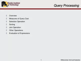
Query Processing • Overview • Measures of Query Cost • Selection Operation • Sorting • Join Operation • Other Operations • Evaluation of Expressions

Basic Steps in Query Processing 1. Parsing and translation 2. Optimization* 3. Evaluation

Parsing, Translation and Evaluation • Parsing and translation: • Checks syntax, verifies relations, attributes, etc. • Translates the query into its internal, relational algebraic form. • Optimization: • Evaluates and compares different ways to implement the query. • Constructs a query-evaluation plan. • Evaluation: • Executes the (chosen) query-evaluation plan. • Returns results. • Our focus will be on optimization…

Optimization • Observation #1 - A given relational algebra expression has many equivalent expressions: balance2500(balance(account)) balance(balance2500(account)) • Observation #2 - Each relational algebraic operation can be evaluated using different algorithms: • Use an index on balance to find accounts with balance < 2500, or • Perform a relation scan and discard accounts with balance  2500

Optimization (Cont.) • Evaluation plan – Annotated relational algebraic expression specifying an evaluation strategy. • a.k.a. query execution plan or query plan • Query optimization – The process of choosing an evaluation plan that has lowest estimated “cost.” • A cost estimate for a plan is calculated using statistical information: • Number of tuples in each relation • Size of tuples • Distribution of attribute values, etc.

Optimization (Cont.) • Query Processing Slides (low-level): • How to measure query cost. • Algorithms for individual relational algebra operations. • How to combine algorithms for individual operations in order to evaluate a complete expression. • Query Optimization Slides (high-level): • How to optimize queries i.e., how to find an evaluation plan with lowest estimated cost.

Measures of Query Cost • Generally, cost can be defined as the total time for query execution. • Many factors contribute to cost: • disk accesses • CPU time • network communication • sequential vs. random I/O • buffer size • writing vs. reading • In database systems the main cost is typically disk access time. • relatively easy to estimate

Measures of Query Cost, Cont. • For simplicity our cost measure will be a function of: • the number of block transfers to/from disk • block access time (seek time + rotational latency) tS • block transfer time tT • buffer size • Real DBMSs take other factors into account.

Measures of Query Cost (Cont.) • The amount of available buffer space depends on several factors: • other concurrent processes, memory size, etc. • Available buffer space is therefore hard to determine in the abstract. • The authors use worst case estimates, assuming only the minimum amount of memory is available for query execution (extremely pessimistic). • Other times they use average case estimates, or a somewhat peculiar mix of average and worst case. • The cost to write the final output to disk is not included in cost estimates.

Statistical Informationfor Cost Estimation • nr: number of tuples in a relation r. • br: number of blocks containing tuples of r. • sr: size of a tuple of r. • fr: blocking factor of r, i.e., the number of tuplesthat fit into one block. • If tuples of r are stored together physically in a file, then:

Statistical Informationfor Cost Estimation • More accurately: • tS : average block access time (seek plus rotational latency) • tT : average transfer time

Selection Operation • Search algorithms that perform selections without using an index are referred to as file scans. • Algorithm A1 - linear search • Scan each block and test all records to see whether they satisfy the condition. • Cost estimate: • Best, worst, and average case tS + br * tT • If the selection is an equality comparison on a cand. key, average case drops to tS + (br /2) * tT • What are best and worst case scenarios? • Linear search can be applied regardless of selection condition, ordering of records in the file, or availability of indices • Note that linear search is sometimes referred to as a table scan or a file scan, although the latter term includes other algorithms.

Selection Operation (Cont.) • Note that the books numbering of the algorithms depends on the edition! • In particular, binary search is not included in the most recent edition. • A2 - binary search • Applicable primarily if selection is an equality comparison, and • Tuples are sorted based on the search key. • Cost: • Assume that the blocks of a relation are stored contiguously • Worst case is log2(br) * (tS + tT) • This is the cost of locating a tuple using a binary search • Plusthenumber of blocks containing records that satisfy selection condition. • Will see how to estimate this cost in the next chapter

Selections Using Indices • Search algorithms that use an index to perform a selection are referred to as index scans. • To use an index, the selection predicate must involve (at least part of) the index search-key. • A3 - primary index on candidate key, equality • At most one record is retrieved. • Cost = (HTi+ 1) * (tS + tT), where HTirepresents the “height” of index i • A4 - primary index on non-key, equality • Zero or more records are retrieved. • Retrieved records will be on consecutive blocks. • Cost = HTi* (tS + tT) + tS + b * tT, where b is the number of blocks containing retrieved records (to be estimated in the next chapter).

Selections Using Indices, Cont. • A5 - equality on search-key of secondary index • Retrieve a single record if the search-key is a candidate key. • Retrieve multiple records if search-key is not a candidate key. • Cost: • If the search-key is a candidate key (single record retrieval): • Cost = (HTi+ 1) * (tS + tT), • If the search-key is not a candidate key (multiple record retrieval): • Cost = (HTi+ n) * (tS + tT), where n = # of records retrieved • Worst case - assumes each record is on a different block • In the next chapter we will develop and estimate for n. • The book does not include block reads for the bucket.

Selections Involving Comparisons • What about selections that aren’t simple tests for equality? • The techniques vary, depending on the complexity of the predicate. • Different vendors will use different “tricks.” • Note that linear search is always a viable option. • For example: AV (r) or A  V(r) • File Scan - linear or binary search (if sorted). • Index Scan - using indices as specified in the following. • A6 - primary index, comparison using or • A  V(r) use index to find first tuple  v and scan sequentially from there. • AV (r) don’t use the index; scan relation sequentially until first tuple > v. • Exercise – give a cost estimate for both of these options.

Selections Involving Comparisons • A7 - secondary index, comparison • A  V(r) use the index to find the first index entry  v; scan the leaves of the index sequentially from there to find record pointers. • AV (r) scan the leaf pages of the index using record pointers, until reaching first entry > v. • Note that both cases requires an I/O for each record, in the worst case. • Exercise – give a cost estimate for both cases.

Implementation of Complex Selections • Conjunction: 1 2. . . n(r) • A8 - conjunctive selection using one index • Select one of the conditions i and algorithms A1 through A7 that results in the least cost for i (r). • Test other conditions on tuples after retrieving them into the buffer. • A9 - conjunctive selection using multiple-key index • Use appropriate composite (multiple-key) index if available. • A10 - conjunctive selection by intersection of identifiers • Use the index corresponding to each condition (if they exist) to obtain sets of record pointers. • Take the intersection of the resulting sets. • Retrieve records from data file. • Pointers could be sorted prior to retrieval (why would you do this???). • If some conditions do not have appropriate indices, apply test in memory.

Algorithms for Complex Selections • Disjunction: 1 2 . . . n (r). • A11 - disjunctive selection by union of identifiers • Use the index corresponding to each condition to obtains sets of record pointers. • Take the union of all the obtained sets. • Retrieve records from data file. • Could sort pointers prior to retrieval. • Applicable only if all conditions have available indices; otherwise use linear scan. • Negation: (r) • Use linear search. • If an index is applicable to , find satisfying records using leaf-level of index and fetch from the data file.

Sorting • Option #1 - Use an existing applicable ordered index (e.g., B+ tree) to retrieve the tuples in sorted order. • Option #2 - Build an index on the relation, and then use the index to retrieve the tuples in sorted order. • Option #3 - For relations that fit in memory, techniques like quick-sort can be used. • Option #4 - For relations that don’t fit in memory, use external sort-merge. • Note that vendors typically have proprietary sorting algorithms.

External Sort-Merge Let M denote memory size (in blocks), and let r be the relation to be sorted. • Create sortedruns: i = 0; while (the end of r has not been reached) { Read M blocks of r into memory Sort the in-memory blocks Write sorted data to disk; label it run Ri; i = i + 1; } N = i; The end result is N runs, numbered 0 through N-1, where each run, except perhaps the last, contains M sorted blocks.

External Sort-Merge, Cont. • Merge the runs (N-way merge): // We assume (for now) that N < M. // Use N blocks, bi, 0<=i<=N-1, of memory to buffer input runs. // Use 1 block, bM, of memory to buffer output. Read the first block of each run into its buffer block; repeat Let t be the the smallest record in sorted order from among all blocks, bi, where 0<=i<=N-1, and suppose that t is in block bk; Write t to bM; if (bM is full) then write bM to disk; Delete t from bk; if (bk is empty) then read the next block (if any) of the run into bk; until all sorted runs are empty;

Original Table • on disk Sorted Runs • on disk • each has M blocks Buffer • Runs are merged block at a time Final Sorted Table • on disk External Sort-Merge(N<M) Sort M blocks in memory R0 Sort M blocks in memory R1 Sort M blocks in memory R2 Sort M blocks in memory RN-1 Output block

External Sort-Merge(N>=M) • If N M, several merge passes are required. • In each pass, contiguous groups of M - 1 runs are merged. • Repeated passes are performed till all runs have been merged into one. • Note: • A pass reduces the number of runs by a factor of M-1, and creates runs longer by the same factor. • E.g. If M=11, and there are 90 runs, one pass reduces the number of runs to 9, each 10 times the size of the initial runs.

Example: External SortingUsing Sort-Merge M=3, and each record takes up 1 buffer block* (very artificial example) R0 R1 R2 R3

External Merge Sort (Cont.) • Cost analysis: • If N < M then total cost is 3br(excluding final output) • If N M then the number of merge passes required is logM–1(br/M) • Block transfers for initial run creation as well as in each pass is 2br • For final pass, we ignore final write cost for all operations. Thus total number of block accesses for external sorting: br ( 2 logM–1(br / M) + 1)

Join Operation • Algorithms for implementing joins: • Nested-loop join • Block nested-loop join • Indexed nested-loop join • Merge-join • Hash-join • Various versions of the above • Choice of algorithm is based on cost estimate. • Examples use the following information: • customer - 10,000 rows, 400 blocks • depositor - 5000 rows, 100 blocks

Nested-Loop Join • To compute the theta join rs // r is the outer relation, s is the inner relation for (each tuple tr in r) for (each tuple tsin s)if (tr and ts satisfy condition ) add tr • ts to the result; • Does not use or require indices. • Can be used with any kind of join condition.

Nested-Loop Join (Cont.) • Worst case – if there are only 3 blocks available, 2 for input, 1 for output – the number of disk accesses is: • nr bs + br • Examples: • 5000  400 + 100 = 2,000,100 with depositor as outer relation. • 10000  100 + 400 = 1,000,400 with customer as the outer relation. • Best case - if both relations fit entirely in memory. • br + bs • If only the smaller of the two relations fits entirely in memory then use that as the inner relation; the bound will still hold. • Example: • 400 + 100 = 500 with depositor or customer as the outer relation.

Block Nested-Loop Join Enhanced version of the nested-loop join: for (each block Br of r)for (each block Bs of s)for (each tuple trin Br)for (each tuple tsin Bs)if (tr and tssatisfy the join condition) add tr• tsto the result; Does not use or require indices. Can be used with any kind of join condition.

Block Nested-Loop Join (Cont.) • Worst case – if there is only 3 blocks available, 2 for input, and 1 for output – the number of block accesses is: br bs + br • Examples: • 100 * 400 + 100 = 40,100 (depositor as the outer relation) • 400 * 100 + 400 = 40,400 (customer as the outer relation) • Best case: br+ bs • Example: • 400 + 100 = 500 (same as with nested-loop join) • Would a nested-loop join ever be preferable?

Improvements to Nested-Loopand Block Nested-Loop Algorithms • Cute little optimizations that only a programmer could love… • For a nested-loop join: Scan the inner relation forward and backward alternately, to make use of the blocks remaining in buffer (with LRU replacement). • For a block nested-loop join: • Use M - 2 disk blocks as the blocking unit for the outer relation, where M = memory size in blocks • Use one buffer block to buffer the inner relation • Use one buffer block to buffer the output • Worst case: br / (M-2)  bs + br • Best case is still the same: bs + br • For either: if the join is an equijoin, and the join attribute is a candidate key on the inner relation, then stop inner loop on first match.

Indexed Nested-Loop Join • Index scans are an option if: • the join is an equijoin or natural join, and • an index is available on the inner relation’s join attribute • For each tuple trin the outer relation r, use the index to look up tuples in s that satisfy the join condition with tuple tr. • Example: • Suppose customer has an index on customer-name. • depositor customer

Indexed Nested-Loop Join • Worst case - the buffer has space for only one block of r and one block of the index for s. • br + nr c, where c is the cost to search the index and retrieve all matching tuples for each tuple or r Worst case will assume index blocks are not in buffer, best case will assume that some are (perhaps close to br+bs if index is pinned in buffer?)

Example of IndexNested-Loop Join Costs • Compute depositor customer, with depositor as the outer relation. • Suppose customer has a primary B+-tree index on customer-name, which contains 20 entries in each index node. • Since customer has 10,000 tuples, the height of the tree is 4, and one more access is needed to find the actual data. • Recall that depositor has 5000 tuples and 100 blocks. • Cost of indexed nested loops join: • 100 + 5000 * 5 = 25,100 disk accesses. Worst case

Indexed Nested-Loop Join, Cont. • Other Options: • If a supporting index does not exist than it can be constructed “on-the-fly.” • If indices are available on the join attributes of both r and s, thenuse the relation with fewer tuples as the outer relation. • Or perhaps use the relation which has a primary index on it as the inner relation…

Merge-Join • Applicable for equijoins and natural joins. • Sort both relations on their join attribute (if not already sorted). • Merge the sorted relations to join them: • Similar to a “classic” merge. • Main difference — every pair of tuples with same value on join attribute must be matched. • Detailed algorithm is in the book. a1 a2a2 a4 a 4 1 c b 4 3 f a 4 4 a c 7 4 d b 7 5 e a 7 5 e d 9 7 d b 9 7 f 8 a 13 c ps pr “gather” “merge”

Merge-Join (Cont.) • Can be used only for equi-joins and natural joins • Best case: • Suppose all tuples for any given value of the join attribute fit in memory. • Each block needs to be read only once. • Thus, the number of block accesses for merge-join is:br + bs + the cost of sorting if relations are unsorted. • Worst Case: • Suppose every tuple from both relations has the same value on the join attribute. • Thus, all tuples for a given value of the join attribute don’t fit in memory. • The algorithm is ambiguous in how it deals with this case. • Block-nested loop is probably the best alternative at this point, in which case the number of block accesses is br + br * bs

Hybrid Merge-Join • Left as an exercise… • Applicable if: • Join is an equi-join or a natural join • One relation is sorted • The other has a secondary B+-tree index on the join attribute • Algorithm Outline: • Merge the sorted relation with the leaf entries of the B+-tree. • Sort the result on the addresses of the unsorted relation’s tuples. • Scan the unsorted relation in physical address order and merge with previous result, to replace addresses by the actual tuples. • Sequential scan more efficient than random lookup. • Not really a “scan” of the whole relation.

Hash-Join • Applicable for equijoins and natural joins. • For the moment, ignore buffering issues… • Let h be a hash function mapping JoinAttrs to {0, 1, ..., n-1}. • h is used to partition tuples of both relations: • The tuples from r are partitioned into r0, r1, . . ., rn-1 • Each tuple tr r is put in partition ri where i = h(tr [JoinAttrs]). • The tuples from s are partitioned into s0,, s1. . ., sn-1 • Each tuple tss is put in partition si, where i = h(ts [JoinAttrs]). *Note that the book uses slightly different notation.

Hash-Join (Cont.) • Tuples in rineed only to be compared with tuples in si: • An r tuple and an s tuple having the same value on the join attribute will have the same hash value. • If that value is hashed to some value i, the r tuple has to be in riand the s tuple in si.

Hash-Join Algorithm • Partition the relation s into n>=1 partitions using hashing function h. // Assume that n<=M-1, for the moment. // When partitioning a relation, one block of memory is used as output for // each partition, and one block is used for input. 2. Partition r similarly. 3. For each iwhere 0<=i<=n-1: (a) Load si into memory // Assume for the moment that it fits, with 2 additional blocks to spare. (b) Read the tuples in ri from the disk one by one (block at a time). - For each tuple tr locate each matching tuple tsin si - Output the concatenation of their attributes. • The hash join of r and s is computed as follows (Preliminary Version):

Hash Join – Partition Phase Table s (on disk) Buffer (M blocks) Partitions of s (on disk) 0 Each consists of “slightly less” than M blocks Input blocks one at a time 1 s0 s1 2 s2 3 Tuples are hashed to buckets n sn-1 *Kind’a like sorting mail or cloths… M-1

Hash Join – Build Phase Partitions of r (on disk) Partitions of s (on disk) r0 s0 r1 s1 r2 s2 ri si rn-1 sn-1

Hash Join – Build Phase Partitions of r (on disk) Partitions of s (on disk) Buffer (M blocks) r0 s0 r1 s1 r2 s2 si will fit because it consists of “slightly less” than M blocks si ri si Input si all at once rn-1 sn-1 M-2 M-1

Hash Join – Build Phase Partitions of r (on disk) Partitions of s (on disk) Buffer (M blocks) r0 s0 r1 s1 r2 s2 si will fit because it consists of “slightly less” than M blocks si ri si Input si all at once rn-1 sn-1 M-2 Input ri block at a time M-1

Hash Join – Build Phase Partitions of r (on disk) Partitions of s (on disk) Buffer (M blocks) r0 s0 r1 s1 r2 s2 si will fit because it consists of “slightly less” than M blocks si ri si Input si all at once rn-1 sn-1 Probe ri with tuples from si to find matching tuples M-2 Input ri block at a time M-1

Hash Join – Build Phase Partitions of r (on disk) Partitions of s (on disk) Buffer (M blocks) Final Result (join) r0 s0 r1 s1 r2 s2 si will fit because it consists of “slightly less” than M blocks si ri si Input si all at once rn-1 sn-1 Probe ri with tuples from si to find matching tuples M-2 Input ri block at a time M-1

Hash-Join Algorithm • Partition the relation s into n>=1 partitions using hashing function h. // Assume that n<=M-1, for the moment. // When partitioning a relation, one block of memory is used as output for // each partition, and one block is used for input. 2. Partition r similarly. 3. For each iwhere 0<=i<=n-1: (a) Load si into memory // Assume for the moment that it fits, with 2+ additional blocks to spare. (b) build an in-memory hash index on the join attribute. // This hash index uses a different hash function than the earlier one h. (c) Read the tuples in ri from the disk one by one (block at a time). - For each tuple tr locate each matching tuple tsin siusing the in-memory hash index. - Output the concatenation of their attributes. • The hash join of r and s is computed as follows: • Relation s is called the buildrelation and r is called the proberelation.

Query Processing