Query Optimization Overview and Statistics Estimation in DBMS
Query optimization involves selecting the most efficient query-evaluation plan for processing a query. Learn about estimating statistics and transformation of relational expressions to optimize database queries effectively.

Query Optimization Overview and Statistics Estimation in DBMS
E N D
Presentation Transcript
Chapter 10 Query Optimization • 10.1 Overview • 10.2 Estimating Statistics of Expression • 10.3 Transformation of Relational Expressions • 10.4 Choice of Evaluation Plans
10.1 Overview Query optimization is the process of selecting the most efficient query-evaluation plan from among the many strategies usually possible for processing a given query. Optimization: ①One aspect of optimization occurs at the relational-algebra level, where the system attempts to find an expression that is equivalent to the given expression, but more efficient to execute. ② another aspect is selecting a detailed strategy for processing the query.
∏customer-name (branch-city=“Brooklyn”(branch (account depositor) ) ) ∏customer-name ((branch-city=“Brooklyn”(branch)) (account depositor) ) ∏customer-name ∏customer-name branch-city=Brooklyn branch-city=Brooklyn account depositor branch branch account depositor 10.1 Overview Find the names of all customers who have an account at any branch located in Brooklyn.
10.1 Overview Given a relational-algebra expression, it is the job of the query optimizer to come up with a query-evaluation plan that computes the same result as the given expression, and is the least costly way of generating the result . To choose among different query-evaluation plans, the optimizer has to estimate the cost of each evaluation plan.(disk access) Generation of query-evaluation plans involves two steps: ① generating expressions that are logically equivalent to the given expression . ② annotating the resultant expressions in alternative ways to generate alternative query evaluation plans.
nr br= fr 10.2.1 Catalog Information The DBMS catalog stores the following statistical information about database relations: nr,the number of tuples in the relation r. br,the number of blocks containing tuples of relation r. lr,the size of a tuple of relation r in bytes. fr, the blocking factor of relation r(that is, the number of tuples of relation r that fit into one block) V(A,r),the number of distinct values that appear in the relation r for attribute A, this value if the same as thesize of∏A(r). If A is a key for relation r,V(A,r) is nr. If the tuples of relation r are stored together physically in a file.
R A B C a b c a b c a a a c c c 4 4 4 1 1 1 . v-min(A,r) nr max(A,r)-min(A,r) 10.2.2 Selection Size Estimation ① A=a(r) : nr/V(A,r) a. uniform distribution of values b. the value a appears in attribute A of some record of r. ② A<=v(r) : Example: ① B=a(r) a. values are uniformly distributed. nr= 6 V(B,r)=2 nr/V(A,r)=3 (1) v<min(A,r) :0 (2) v>= max(A,r) : nr ① C<=3(r) (3) min(A,r) <v <= max(A,r) : nr= 6 min(A,r)=1 max(A,r)=4 6*(3-1)/(4-1)=4
i (r) For each i we estimate the size of the selection , denoted by si. Thus, the probability that a tuple in the relation satisfies selection condition is si/nr. (selectivity of the selection ) i (r) R A B C . a b c a b c a a a c c c 4 4 4 1 1 1 . . . . S1 S2 . nr = S1 S2 … Sn nr 2 n nr nr 10.2.2 Selection Size Estimation ③ complex selections: a. Conjunction: 1∧ 2∧… ∧ n(r) Assuming that the conditions are independent of each other. a. B=a ∧ C<=3(r) B=a (r): 3 C<=3 (r): 4 6*(3*4)/6*6=2
. S2 S1 S1 S2 Sn nr (1-(1- )(1- )(1- )) nr nr nr nr nr (r) (r) nr- nr- R . A B C nr (1-(1- )(1- )) a b c a b c a a a c c c 4 4 4 1 1 1 c. B=a (r) =6-3=3 10.2.2 Selection Size Estimation 1 ∨2 ∨ … ∨n(r) b. Disjunction: let si/nr denote the probability that a tuple satisfies condition i. b. B=a ∨ C<=3(r) B=a (r): 3 C<=3 (r): 4 ¬(r) c. Negation: =6*(1-(1-3/6)(1-4/6))=5 B=a (r): 3
① If R∩S= ,then r s is the same as r×s,and we can use our estimation technique for Cartesian products. ② If R∩S is a key for R, then we know that a tuple of s will join with at most tuple from r. therefore, the number of tuples in r s is no greater than the number of tuples in s. if R∩S forms a foreign key of S, referencing R, the number of tuples in r s is exactly the same as the number of tuples in s. 10.2.3 Join Size Estimation The Cartesian product r×s contains nr * ns tuples, each tuple of r×s occupies lr+ls bytes. Let r(R) and s(S) be relation:
ns V(A,s) nr *ns nr *ns V(A,s) V(A,r) 10.2.3 Join Size Estimation ③ when R∩S is a key for neither R nor S. we assume that each value appears with equal probability. Consider a tuple t of r, and assume R∩S ={A}. We estimate that tuple t produces tuples in r s. Considering all the tuples in r, we estimate that there are tuples in r s. If we reverse the roles of r and s in the preceding estimate, we obtain an estimate of These two estimates differ if V(A,r) = V(A,s). The lower of the two estimates is probably the more accurate one.
Example: Depositor-schema=(customer-name, account-number) Consider the expression depositorcustomer Customer-schema=(customer-name, customer-street, customer-city) Assume the following catalog information about the two relations: 10.2.3 Join Size Estimation bcustomer= ncustomer /fcustomer =400 ncustomer=10000 fcustomer=25 bdepositor= ndepositor /fdepositor =10 ndepositor=5000 fdepositor=50 V(customer_name,depositor)=2500 Assume that customer-name in depositor is a FK on customer According to ②the size of the result is ndepositor=5000
nr* ns nr* ns 5000*10000 5000*10000 = = =5000 V(A,s) V(A,r) 2500 10000 = = =20000 ndepositor*ncustomer ndepositor*ncustomer V(customer-name,depositor) V(customer-name,customer) 10.2.3 Join Size Estimation Without using information about FK.According to③ We choose the lower one 5000.
10.2.4 Size Estimation for Other Operations ①Projection: the estimated size of a projection of the form ∏A(R) is V(A,r). Since projection eliminates duplicates. ②Aggregation: the size of a projection of AGF(r) is simply V(A,r). Since there is one tuple in AGF(r) for each distinct value of A. ③Set operations: if the two inputs to a set operation are selections on the same relation, we can rewrite the set operation as disjunctions, conjunctions, or negations. Example:1(r)∪2(r) can be rewritten as1∨2(r) 1(r)∩2(r) can be rewritten as1∧2(r) 1(r)-2(r) can be rewritten as1∧¬2(r)
a.rs the size of r s+ the size of r b.rs the size of r s+ the size of s c.rs the size of r s+ the size of r+the size of s 10.2.4 Size Estimation for Other Operations if the inputs are not selections on thesame relation we estimate the sizes this way: a.r∪s the sum of the sizes of r and s b.r∩s the minimum of the sizes of r and s c.r-s the same size as r ④Outer join:
For selections, the number of distinct values of an attribute A in the result of a selection, V(A, ), can be estimated in these ways: (r) ①If the selection condition forces A to take on a specified value (e.g.,A=3), V(A, )=1 (r) ②If forces A to take on one of a specified set of values (A=1∨A=3 ∨A=4), then V(A, )is set to the number of specified values. (r) (r) ③If the selection condition is of the form A op v, V(A, ) is estimated to be V(A, r)*s, where s is the selectivity of the selection. ④In all other cases of selections, we assume that the distribution of A values is independent of the distribution of the values on which selection conditions are specified, and use an approximate estimate of min(V(A,r), ). n(r) 10.2.5 Estimation of Number of Distinct Values
1. Conjunctive selection operations can be deconstructed into a sequence of individual selections. (a cascade of ) 3. Only the final operations in a sequence of projection operations are needed, the others can be omitted. (a cascade of ) ∏ 10.3.1 Equivalence Rules An equivalence rule says that expressions of two forms are equivalent. 1∧2(E)= 1 (2(E)) 2. Selection operations are commutative. 1 (2(E))=2 (1(E)) ∏L1(∏L2 (…(∏Ln(E))…)) =∏L1(E)
(E1×E2))= E1 E2 1(E12E2))= E1 1∧2E2 b. E1E2= E2 E1 (E1E2) E3 =E1 (E2 E3) (E11E2) 2∧3E3 =E1 1∧3(E2 2E3) 10.3.1 Equivalence Rules 4. Selections can be combined with Cartesian products and theta joins. a. 5. Theta-join operations are commutative. 6. a. Natural-join operations are associative. b. Theta joins are associative in the following manner:
0(E1E2))=(0(E1))E2 1∧2 (E1 E2) = (1(E1)) (2(E2)) 10.3.1 Equivalence Rules 7. The selection operation distributes over the theta-join operation under the following two conditions: a. It distributes when all the attributes in selection condition 0 involve only the attributes of one of the expressions(say, E1) being joined. b. It distributes when selection condition 1involve only the attributes of E1and 2 involve only the attributes of E2
∏L1∪L2(E1E2))= (∏L1(E1)) (∏L2(E2)) b. Consider a join E1 E2. Let L1 and L2 be sets of attributes from E1 and E2, respectively, let L3 be attributes of E1 that are involved in join condition , but are not in L1∪L2, and let L4 be attributes of E2 that are involved in join condition , but are not in L1∪L2. Then, ∏L1∪L2(E1E2))=∏L1∪L2((∏L1∪L3(E1)) (∏L2∪L4(E2))) 10.3.1 Equivalence Rules 8. The projection operation distributes over the theta-join operation under the following conditions: a. Let L1 and L2 be attributes of E1 and E2, respectively. Suppose that the join condition involves only attribute in L1∪L2. Then,
10.3.1 Equivalence Rules 9. The set operations union and intersection are commutative. E1∪E2 =E2∪E1 E1∩E2 =E2∩E1 10. Set union and intersection are associative. (E1∪E2)∪E3 =E1∪(E2∪E3) (E1∩E2)∩E3 =E1∩(E2∩E3) 11. The selection operation distributes over the union, intersection, and set-difference operations. P(E1-E2)=P(E1)-P(E2) ∪∩ P(E1-E2) =P(E1)-E2 ∩ 12. The projection operation distributes over the union operation. ∏L (E1∪E2)=(∏L1(E1))∪(∏L(E2))

