Download
1 / 51
540 likes | 806 Vues
Water Budget III: Stream Flow. P = Q + ET + G + Δ S. Why Measure Streamflow ?. Water supply planning How much water can we take out (without harming ecosystems we want to protect) Flood protection How much water will come down the channel if X storm happens? Who’ll be flooded?

E N D
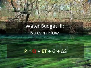
Water Budget III: Stream Flow P = Q + ET + G + ΔS
Why Measure Streamflow? • Water supply planning • How much water can we take out (without harming ecosystems we want to protect) • Flood protection • How much water will come down the channel if X storm happens? Who’ll be flooded? • Water quality • What are the fluxes (flow x concentration) of contaminants to a lake or estuary? • What are the effects of land use change on water delivery to downstream systems?
Extreme Low Flows Rainfall between Oct 1. 2010 and January 21, 2011 is 2.68 inches
Watersheds as Filters • Rain falls • Storages “buffer” the rainfall signal, letting water out slowly • More storage = more buffering • The result is that the rainfall signal looks stochastic, the flow looks more “organized” • Watershed properties AND size affect the filtering effect
Consider the “Filter” Effects of: • Watersheds with steep vs. shallow slopes • Watersheds with deep vs. shallow soils • Watersheds with intense vs. extended rainfall • Watersheds with forests vs. parking lots • Watersheds with dams vs. not • Big vs. little watersheds • Watersheds with big shallow aquifers
Where is Stream Flow From? • At any time, flow is a composite of water with different sources and residence times • Some water is stored in the watershed for a very long time, some very short • During low flow conditions, water is mostly old • During storms, the contribution of new water increases • How does an aquifer affect this?
23% 8% 2%
Flow and Rainfall Intensity • If Rainfall Intensity > Infiltration Capacity then surface runoff occurs • Stream flows are composites of • Surface runoff • Subsurface flows
Land Use (Cover) Affects Runoff Generation • Impervious surfaces preclude infiltration • Less infiltration means more runoff • Runoff also MOVES faster • Less “filtering” • Compare land uses…
Forest Ag Urban
The importance of storage – the basis of filtering Same total flow (area under the curve), lower peak flow.
Wetland Hydrological Services Depressions and vegetation (swamps) slow runoff. Upper watershed wetland storage delays runoff and reduces peak flows. Wetland flood plain has a dominant influence on downstream peak flow and solute transport.
Why Does Storage Matter? 200,000 m3 of Stormwater Runoff; Channel Peak Flow capacity of 1m3/s All in one day Peak Flow =2.3 m3/s Spread over 3 days Peak Flow = 0.8m3/s
How Big a Flood Can We Expect? • The size of the flood is inversely proportional to it’s frequency • Big event happen rarely • Big events shape the landscape • Medium events maintain the landscape • Small events control the biology • How would we predict the size of a flood that happens roughly once in 25 years? • Think back to the rainfall lab…
How Do We Measure Streamflow? • Funny you should ask…basis of Lab #4. • Basis is to estimate: • Cross-sectional area (A; through which water flows) • Water flow velocity (V) • Q = A * V
Where to measure mean velocity? Float Velocity * 0.8 for natural channels Float Velocity * 0.9 for concrete channels
Velocity Instruments $2k Turn-cup 0.500 ft/s $4k $7k Electromagnetic 0.050 ft/s Sonic Doppler 0.005 ft/s
Discharge is HARD to Measure • We want: • Daily (or sub-daily) measurements • Multiple stations per river • Real time updating (detect changes in flow as they are happening)
Rating equations (stage vs. discharge) allow continuous flow monitoring
Stage-Discharge Relation • Water stage (elevation) is EASY to measure • Stage is related to dischage via a mathematical relationship • Applying that relationship to measured stage gives estimates of discharge H H Q t t Q Stage-Discharge Curve or Rating Curve Discharge Hydrograph Stage Hydrograph
Stage-Discharge Relation • Typical relationship: Q = a(H +b)c • The relationship between H & Q has to be calibrated locally for different stations
Stage Discharge Relationship for the Ichetucknee River • At low stage, positive relationship between stage and discharge • At high stage, negative relationship • Why? Discahrge Stage
Stage Measurements Float-pulley Staff gage Ultrasonic Pressure
What if there’s no rating curve? • New watershed, new conditions • Areas where it’s hard to develop rating curves • For example, the Everglades
Manning’s Equation - Flow Estimation without a rating equation Q= 1/n * A * r 2/3 * s1/2 Q = estimated flow m3/s n = Manning’s roughness number (0.02 smooth to 0.15 rough or weedy, 0.5 dense vegetation) A = cross sectional area (m2) r = Hydraulic Radius (wetted perimeter = WD/(W + 2D) W > 10D, R → D) s = Hydraulic Gradient ΔH/L
Predicting Flow in the Everglades • Dense vegetation channel (n = 0.4) • Shallow slope (s = 3 cm per km = 0.00003) • Wide channel (100 m wide, 0.3 m deep, A = 30 m2, r = 30 m2 / 100.6 m = 0.3 m) • What is Q? What is flow velocity (u)? • Q = (1/n) * A * r0.67 * s0.5 • V = Q / A • Q = (1/0.4) * 30 m2 * 0.3 m0.67 * 0.000030.5 = 0.183 m3/s • V = 0.183 m3/s / 30 m2= 0.006 m/s = 0.6 cm/s