Download
1 / 31
310 likes | 334 Vues
This paper explores quantum impact in collisional broadening, discussing various impact models and the transition from impact theory to simulations. The Lorentz model, perturbations on emitters, and the Quantum Uncertainty Principle are analyzed along with the validity conditions of impact approximation. The study delves into calculations for perturbers as wave packets and classical versus quantum impact models, highlighting advancements in the field and areas requiring further analysis. Collaboration between research institutions and applications in astrophysics are also discussed.

E N D
Stark broadening from impact theory to simulations R. STAMM1 I. HANNACHI2, M. MUREINI1, L. GODBERT-MOURET1, M. KOUBITI1 Y. MARANDET1, J. ROSATO1 M. DIMITRIJEVIC3 and Z. SIMIC3 1 Physique des Interactions Ioniques et Moléculaires Aix-Marseille université / CNRS 2 University Batna 1 3 Astronomical Observatory, Belgrade, Serbia 11th SCSLSA
Outline Introduction Different impact models Beyond impact Conclusion
Collision and radiation, Lorentz profile perturber Atom (emitter) Light emission (frequency w0) Lorentz model : the perturber cuts the light waveW(t)= exp(iw0t) as itgetsnear to the emitter (collision) EmitterW(t)starts at t=0, ends at t=t (average time betweenstrong collisions) Power spectrumI(w)=W(w) W*(w): Lorentz profile collisionnalbroadening
Quantum mechanics Uncertainty principle. An energy level above ground state with energy E and lifetime Δt has uncertainty in energy: States which are short-lived have large uncertainties in the energy. This is natural broadening and leads also to a Lorentzian profile Reducing the lifetime of a state broadens the spectrum of the emitted line But broadening can be done gradually, each perturbation changing e.g. the phase of the light dephasing effect collision
Nonbinary quantum calculation or impact approximation? Starting point : dipoled of the emitter The effect of perturbations is a change of the emitted radiation. This canbemeasured by the dipoleautocorrelationfunction (DAF) of the emitter T(t) emitter evolution operator, r density matrix Trace over all possible states of the quantum system emitter plus perturbers Could be calculated by density functional theory or quantum Monte Carlo methods (density functional method, quantum Monte Carlo) But for a large range of conditions: -Collisions are binary -Collision time is much larger than the time of interest (inverse of line width) These are the validity conditions of the impact approximation
Outline Introduction Different impact models Beyond impact Conclusion
Quantum impact for emitter and perturbers Perturbers as wavepackets Each wave packet is scattered in the interaction potential with the emitter Started in 1970 (Barnes and Peach, Bely and Griem) Calculation for isolated lines of ions, with an expression using the optical theorem: where N is the perturbers density, v their velocity, and si and sfare inelastic cross sections, fiand ff the forward scattering amplitudes in a direction given by q, j for the initial i and final f states. New life today for suchcalculations (Elabidi, Sahal-Bréchot, Dimitrijević), often in agreement withothermethods
Isolated lines: efficient semi-empirical model Makes use again of the expression using the opticaltheorem Bethe-Born approximation for evaluating inelastic cross sections Width expressed with a Gaunt factor (a quantity which measures the probability than an incident electrons changes its kinetic energy ) Numerouscalculationperformed for isolated ion lines of astrophysicalinterest Dimitrijević and Konjević. Collaboration Belgrade-Marseille Resultsallowedmany diagnostic applications
Classical path approximation, ion lines Perturbersfollow a classicaltrajectory Valid if the wavepacketremainswelllocalized in space For isolated lines, the semi classical perturbation method (SCP) has been applied successfully to many kinds of emitters (Dimitrijević, Sahal-Bréchot) Inspired by all the developments of the quantum theory of collisions (Clebsch-Gordan averages) Accuracy generally better than 20 to 30% for the width. Method continuously improved, and interfaced with atomic structure codes Collaborations: Meudon observatory, ICSLS, since 1980’s
Classical versus quantum impact calculations Quantum calculations have often been found to predict narrower lines than those of semiclassical models Semiclassical calculations may be brought closer to quantum widths, e.g. by a refined calculation of the minimum impact parameter allowing the use of a classical path Surprisingly, quantum widths of Li-like and boron-like ions often show a worse agreement with experiments than semiclassical calculation, thus calling for further calculations and analysis Collaboration: SLSP
Outline Introduction Different impact models Beyond impact Conclusion
Beyond Standard model (impact electrons and static approximation for ions) not validated by accurate hydrogen line profile measurements in arc plasmas (nineteen seventies) Problems in the line centers, and also in the far wings. -line wings well reproduced by unified theory -The observation of the Lyman a line 40 years ago showed that the experimental profile is a factor 2.5 broader than the theoretical line using static ions in arc plasma conditions. Grützmacher K. ; Wende B. Discrepancies between the Stark–broadening theories of hydrogen and measurements of Lyman aStark profiles in a dense equilibrium plasma Phys. Rev. A1977, 16, 243-246.
Alternative Stark broadening models Ion dynamics models No analytic solution Use of stochastic processes: -model microfield method (MMM), Stehlé, C. Astrophys., Suppl. Ser. 1994, 104, 509-527. -Frequency fluctuation model, Talin et al. Phys. Rev. A1995, 51, 1918-1928 Thesemodels use statisticalproperties of the microfield (PDF, <E(0)E(t)>) -Use of a numerical simulation for the microfieldcoupled to a numericalintegration of the emitter Schrödinger equation Periodicboundary conditions or recyclingboundary conditions
Numerical simulation One component of the electricfieldduring the time of interest of Lymana (La) Binary condition : Weisskopf radius << r0 ,here
Numerical simulation Dipole autocorrelation function (DAF) for Lyman a (La) Integration over 3000 field histories for the Ab-initio numerical simulation
Numerical simulation One component of the electric field during the time of interest of Balmer b (Hb)
Numerical simulation Dipoleautocorrelationfunction (DAF) for Balmer b (Hb) Integration over 3000 field histories for the Ab-initionumerical simulation
Numerical simulation In near impact conditions, thereisalways a background of electric field fluctuations with a magnitude of about E0 or and a typical time scale longer than the collision time r0/vi. Such fluctuations correspond to the sum of electric fields of distant particles. For hydrogen lines affected by linear Stark effect, it is well known that this effect of weak collisions is dominant in near impact regimes and results from the long range of the Coulomb electric field. (Griem). Integration over 3000 field histories for the Ab-initionumerical simulation
Line shapewith Langmuir waves Plasmas sustain various types of waves which behave differently in a linear and nonlinear regime. A way to distinguish between the two regimes is to calculate the ratio W of the wave energy density to the plasma energy density, given by Baranger & Mozer, Phys. Rev. 123, 25 (1961), predict the observation of satellites at PavleSavic collaboration Serbie-France (Dimitrijević,Simić)
Simulation for linear waves One electricfield history corresponds to one Langmuir wave with a given electric field direction, magnitude and phase The dipole autocorrelation function (DAF) is obtained after an average over thousand field histories We integrate the Schrödinger equation retaining the impact broadening of the background plasma, plus the waves For La, Ne=1019 m-3, T=105 K, and W=0.01 (EL=15 E0) Response of the DAF: oscillation with period 2p/wp, but almost not visible
Langmuir rogue waves? We assume the presence of an external perturbation, e.g. a beam of chargedparticles Nonlinearphenomena: coupling of the Langmuir, ion sound and electromagneticwaves Background of low magnitude Langmuir waves, but a significant fraction of the wave has a larger magnitude (3 times the background wave magnitude, W =0.1) Rogue waves are a unifying concept for studying Localized excitations, which exceed the strength of the background structures
The creation of rogue vagues Rogue waves in plasma: surface plasma, dusty plasma, electron-positron plasma -Modelingmostoften uses the NonlinearSchrödinger equation One dimensional solution : stable soliton, e.g. Peregrinesoliton
Toy model for Langmuir rogue waveeffect on La Weadd in our Langmuir wave simulation the effect of rogue waveswithEL=45 E0 (3 times the magnitude of the linear wave, with W=0.1, Lorentzian envelope soliton)
Rogue waveeffect on La Weadd in our Langmuir wave simulation the effect of rogue waves
Summary -Line shapescanoftenbedescribedusing an impact approximation -Manydifferentmodels use the impact approximation -Ab initiosimulations canreproduce the impact profiles -Impact broadeningscreensothereffectslikewaveeffects
Collaborations -Started long time agowith Milan Dimitrijevic -Collaboration on the Stark broadeningformalism -Collaboration on diagnostics -Role of SCSLSA: enabled discussions betweenthe different groups and countries -ManyThanks to Milan and all colleagues
Electric field history Average peak field 100 E0, jumping frequency n=wp/50 plasma T= 104 K, Ne=1013 cm-3 Lorentzian envelope functions Sj(t) with a time width DTL 40% of t
Calculation of the dipole autocorrelation function D is the emitter dipole, U(t) the evolution operator is obtained by solving the Schrödinger equation This is done numerically for a history of The dipole autocorrelation function (DAF) is obtained after an average over all configurations of the turbulent Langmuir field In the following we average over 104 field histories
Stark broadening: the line shape Fourier transform of the dipole autocorrelation function (DAF) Different calculations are possible -The single effect of strong Langmuir turbulence (pure Langmuir) -The effect of equilibrium Stark broadening (pure Stark) -The result of a convolution of the the two previous (full profile)
Lya DAF, effect of the envelope shape DTL t Ratio of the Lorentzian half width DTL to the duration t of a step (here about 50 %)
Collision time Static and impact approximations Two limiting regimes Static: Time of interest Only the PDF P(E) is needed Impact: Binary collisions (electrons)