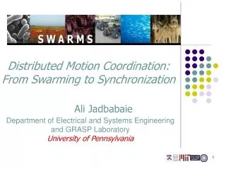
Distributed Motion Coordination: From Swarming to Synchronization
440 likes | 464 Vues
This seminar explores the emergence and sustainability of coordinated group behavior in flocks, swarms, and schools. The seminar also discusses the conditions for reaching consensus in multi-agent systems and the synchronization of coupled oscillators.

Distributed Motion Coordination: From Swarming to Synchronization
E N D
Presentation Transcript
Hamilton Institute Seminar 06/24/2005 Distributed Motion Coordination:From Swarming to Synchronization Ali Jadbabaie Department of Electrical and Systems Engineering and GRASP Laboratory University of Pennsylvania
Distributed Coordination in nature • Flocks, swarms and schools exhibit coordinated group behavior although each animal acts completely autonomously • How do these behaviors emerge? • How are they sustained? • How do individual decisions lead to collective group behavior? SWARMS
Complexity, Statistical Physics, emergence of collective behavior SWARMS
r neighbors of agent i agent i Vicsek’s kinematic model • How can a group of moving agents collectively decide on direction, based on nearest neighbor interaction? How does global behavior emerge from local interactions? SWARMS
= speed MAIN QUESTION :Under what conditions do all headings converge to the same value and agents reach a consensus on where to go? = heading Distributed consensus algorithm SWARMS
Multi-agent Representations: Proximity Graphs We use graphs to model neighboring relations • V: A set of vertices indexed by the set of mobile agents. • E: A set of edges the represent the neighboring relations. • W: A set of weights over the set of edges. Agent i’s neighborhood The neighboring relation is represented by a fixed graph G, or a collection of graphs G1, G2,…Gm SWARMS
switching signal , adjacency matrix finite set of indices corresponding to allgraphs overnvertices. Valence matrix Vicsek’s model 4 3 5 2 6 1 SWARMS
Conditions for reaching consensus Theorem (Jadbabaie et al. 2003): If there is a sequence of bounded, non-overlapping time intervals Tk, such that over any interval of length Tk, the network of agentsis “jointly connected ”, then all agents move in a formation. This happens to be both necessary and sufficient for exponential coordination, boundedness of intervals not required for asymptotic coordination. (Moreau ’04, Ren & Beard ‘05) SWARMS
Extensions • Asynchronous update (Tsitsiklis et al. ‘84,Cao and Morse ‘04) • Switching, directed graphs (Moreau ’04, Ren & Beard’04, Zhu, Francis ’04) • Gossip in networks ( Boyd et a. ’04) • Balanced, directed graphs, no switching.Olfati & Murray 04 • Consensus +quantization (Savkin ’04). • Consensus on random graphs (Hatano and Mesbahi ’04) • No quadratic Lyapunov function exists, but maxji – minjj is a valid Lyapunov function, if connectivity holds. (products of length n-1 of Fi s are pseudo-contractive with respect to a subspace norm. ) • Analysis extends to Choose x = tan() SWARMS
Motion Coordination with Dynamic Models • Double integrator model • Neighbors of i: SWARMS
The control law • The control law has two components: • cohesion/separation input • synchronization input SWARMS
Pair wise attraction and repulsion potentials • Each Vij is required to be: • increasing as • unbounded as • unique minimum • The potential energy Vi of boid i depends on its neighbors Example (Ogren et al ’04, Fiorelli and Leonard ’02) SWARMS
The Laplacian of the graph • The graph Laplacian encodes structural properties of the graph • Some properties of the Laplacian: • It is positive semi-definite • The multiplicity of the zero eigenvalue is the number of connected components • One corresponding eigenvector is the vector of ones, 1. • The second smallest eigenvalue quantifies connectivity. SWARMS
Dynamic Topology Local sensing/communication Graph changes with time Control is discontinuous Non smooth Lyapunov theory Fixed Topology Fixed (logical) network Graph is constant Control is smooth Classic Lyapunov theory Topology dictates analysis SWARMS
For both fixed and dynamic topology:If the neighboring graph stays connected, all agent velocity vectors become asymptotically the same, collisions between interconnectedagents are avoided and the system approaches a configuration that minimizes all agent potentials. Conditions for coordination We could shape potentials for any desired configuration, and also update it as the objective changes. SWARMS
History of the coupled oscillators • Study of Mutual synchronization of biological oscillators goes back to Weiner in 1950s . • Examples: pacemaker cells in the heart and nervous system, collective synchronization of pancreatic beta cells, synchronously flashing fire flies. • Synchronization of oscillators has also been studied in the context of injection locking in RF circuits • Good abstraction for studying networks of loads and generators in the power grid. • All-to-all case with infinite oscillators characterized, finite case and arbitrary topologies open … See the book by Steven Strogatz SWARMS
Synchronization of coupled oscillators • Consider a group of N oscillators coupled nonlinearly as • It is the simplest model of coupled oscillators, simple enough for analysis, but complicated enough to have interesting non-trivial behavior. • The degree of synchronization, is measured with the magnitude of the average phasor: • r(t) close to 1 means synchronization, and r(t) close to zero means asynchrony. How can we extend this to arbitrary interconnections? SWARMS
Laplacian & Incidence Matrix 1 B is the (n x e) incidence matrix of graph G. 2 • Weighted Laplacian • Some properties of the Laplacian: • The e dimensional vector space of edges can be decomposed to an n-1 dimensional cut space(span of columns of BT) and m-n+1 dimensional cycle space(Kernel of B). 3 4 W is diagonal SWARMS
Kuramoto model with incidence matrices B is the incidence matrix of the graph representing the interconnection of oscillators Simple case: all oscillators are identical Theorem:Consider the unperturbed Kuramoto Model defined over an arbitrary connected graph with incidence matrix B. For any given 0 and any positive value of the coupling, the vector is a locally asymptotically stable equilibrium solution. Furthermore, the rate of approach to equilibrium is no worse than SWARMS
A Special Case Thus For |i|</2 for a connected graph, all trajectories will converge to S Therefore, all velocity vectors will synchronize. But, this stability result is not global. In the case of the ring topology is not the only equilibrium. This is due to the fact that B and BT have the same null space! is also stable: Fixed points: SWARMS
Properties of the model • When =0, is an asymptotically stable fixed point. • The order parameter can be written as Where e is the number of edges in the graph • is a Lyapunov function, measuring velocity misalignment. • Using LaSalle, all trajectories converge to invariant sets. Can extend to the case of changing topology, if the graph is “jointly connected”. • The speed of synchronization depends on the algebraic connectivity of the graph (2nd smallest eigenvalue of the Laplacian). SWARMS
Onset of Synchronization • When the frequencies are non zero, there is no fixed point for small values of coupling. • Theorem:Bounds on the critical value of the coupling can be determined by maximum deviation of frequencies from the mean, and algebraic connectivity of the graph. • When is random, • Can develop a mean field model for general topologies by SWARMS
Sum of pair-wise potentials Supply at each node Subject to: Lagrangian Dual decomposition and nonlinear network flow • Want to globally minimize 1-r2 over the whole network • Let z= sin(BT) Kuramoto model is the Subgradient algorithm for solving the dual Shor 87, Tsitsiklis ’86 Subgradient algorithm SWARMS
Kuramoto model with non-homogeneous delays • Phase information from neighbors arrive with arbitrary time delay ij<1. [Aij] is the adjacency matrix. • In case of degree regular graphs, linearized model with ij= was studies by Earl and Strogatz • Using Lyapunov-Krasovskii functionals, can analyze the case of arbitrary connected graphs and non-homogeneous delays. • We assume K is large enough that the oscillators are synchronized, and linearize the dynamics around the synchronized state, i(t) = , where i = t + i(t) • with Gij = Aij cos( ij) SWARMS
Delay Independent Stability • Theorem: Consider a network of N identical oscillators with linearized dynamics Gij = Aij cos( ij)and Gij>0 when i and j are neighbors. Synchronized state is stable independent of delay. Proof sketch: Usethe following V() as a Lyapunov/Krasovski functional : Corollary:If [Gij] is the adjacency matrix of a connected graph, then the continuous time, consensus problem is asymptotically stable with arbitrary time delays SWARMS
Biologically plausible coordination for kinematic robots The input Minimizes the misalignment potential The control law minimizes the potential by following its gradient. But we can’t measure the headings of neighbors W/O communication SWARMS
Yw qj j lij qi bij i Xw Biologically plausible sensing Knowing relative heading would mean having binocular vision or solving structure from motion. This would require multiple visible features on each agent. Measured Quantities • the projection of an agent (bearing) βij • the speed of the projection (optical flow) • The time-to-collision or Expansion rate (rate of approaching or receding of an object), measured as the relative rate of change of the projection area Pigeons and flies are capable of all 3 measurements!. Wang & Frost, Nature, 1992, Fry and Dickinson , Science 2003 SWARMS
A distributed control law • Theorem: with the distributed controller joint connectivity in time flocking Proof based on construction of Lyapunov function whose derivative is the quadratic form of a state dependent Laplacian, and the following lemma SWARMS
Agent i’s neighborhood Coordination in 3D Consider a group of N agents with different velocity vectorsand constant, unit speed (extension to dynamic case possible). θ is the heading and φ is the attitude. SWARMS
Zw TiS X iq vj aij vi X if Xw Yw Geodesic Control Law Bullo, Murray and Sarti, “Control on the Sphere and Reduced Attitude Stabilization”, 1995 SWARMS
Zw TiS Yij Xq vj vi Xf Yw Geodesic Versor For any two agents iand j : • Geodesic versor Yij shows the geodesic direction from vi to vj is the component of vj orthogonal to vi. aij Xw SWARMS
Zw TiS Yij Xq vj vi Xf Xw Theorem [ Moshtagh, Jadbabaie and Daniilidis, CDC’05]: Consider the system of N equations If the proximity graph of the agents is fixed and connected, then the control laws result in flocking. Furthermore the consensus state is locally asymptotically stable. A similar result holds in the case of switching graphs, if the union graph is connected in time. aij Yw SWARMS
Lyapunov function: measure of discrepancy between velocity vectors velocity vectors will synchronize. Lyapunov-based proof In 2-d this is vT L v It Can be shown that Using LaSalle’s invariance principle, all trajectories converge to the largest invariant set within the set: For 0<|i|<, could also use ||||^2 as a Lyap. Function. For a sublevel set inside |i|</2, all trajectories converge to a set where i =j Use ||||^2 as Lyapunov function on this set, then all trajectories will converge to SWARMS
vj Qij Vision-based control law generalizes to 3D Visual Servoing Approach Equation of Motion Agent i We can solve for the input in terms of the measurements. We can construct distributed control laws for flocking, based on visual sensing and measurement of bearing, time to collision and optical flow. No communication or relative distance or heading information is needed SWARMS
Current Research Simulations Leader following Leaderless SWARMS
Research Issues • Implementation on ER robots (underway!) • Measurement of OF and TtoC is noisy!! (How do flies do it?) • How to optimize connectivity in a distributed way? Use 2(L(x)) =0 as an obstacle • 2(L(x)) is matrix concave!!, the corresponding eigenvector gives a subgradient direction • 2(L+L) ≥2(L)+Trace(G L), G=v2 v2* , Lv2=2 v2 • Can find v2 in a distributed way!! • How does the graph evolve as a function of the positions? • Potential-based forces can be used for collision avoidance, but how can we avoid local minima in graphs with cycles? • Determine which edges have the most impact on 2(L) SWARMS
Another example: Geographic routing w/o location info Routing algorithms find best paths for sending messages from sources to destinations in a multi-hop fashion In geographic routing nodes have GPS, and know each other’s location. Messages are passed to the neighbor which is closest in distance to the destination. Scalable to large nodes, but requires location information. In a recent paper,(Rao, Anaswamy, Papadimitriou, Shenker, Stoica, MOBICOM 2003), propose a routing algorithm W/O location information. SWARMS
Rao et al.’s algorithm • Choose virtual coordinates for nodes and perform greedy routing • Proceed closer to destination at each hop. • Assume only perimeter nodes of the network know their correct (relative) locations and are fixed. • Other nodes compute coordinates by averaging with nearest neighbors. • Repeat until convergence, use these coordinates for routing. SWARMS
4 5 3 2 6 1 Updating Virtual coordinates by averaging Peripheral nodes Internal nodes Define a graph to represent proximity relation for internal nodes nodes There is an edge if two nodes are neighbors Laplacian adjacency matrix: Valence matrix SWARMS
What is the corresponding optimization? • The algorithm is providing a minimum energy embedding. • Find pi such that • Minimum corresponds to the kernel of the Laplacian of the whole graph SWARMS
Main Result Theorem: Iteration converges if the graph is connected. The final location of the internal nodes is in the interior of the convex hall of peripheral nodes. Final value depends on the inverse of a diagonally perturbed Laplacian In non-negative matrix theory, this is called an inverse-M matrix For connected graphs, (i.e., A irreducible), this inverse is symmetric positive definite and positive element-wise (totally positive). Gives interesting information about “resistance” or “bottlenecks” in the graph SWARMS
Resistance Distance (RD) • The coefficients of the convex combination depend on the resistance distancebetween each internal node and the peripheral nodes. • Resistance distance, is the open circuit resistance between two nodes of a graph, if all edges are 1 ohm resistors. • It can be calculated from any generalized inverse of the Laplacian as • RD is robust to perturbations in graph • The distributed averaging algorithm is effectively providing a measure of distance between each internal node and the peripheral nodes via RD. • on a random walk. • When the graph is a tree, this reduces to regular hop count (geodesic) distance. Network flow interpretation:Rij is the min-norm flow when unit flow enters from i and leaves from j. SWARMS
More on resistance distance • While Routing based on Euclidean distance might not provide information about graph topology, routing based on resistance distances does! • This seems to be the reason for the good performance of the algorithm, compared to Geographic routing with locations. • The matrix (D-A+B)-1 is a Gramm matrix for set of points realizing resistance distances (Fiedler ’98) • Same is true for pseudo inverse of L. • Resistance distance was (re) introduced by Klein in the context of study of molecular conformations (Klein & Dandic’93). SWARMS
