Clock Synchronization
Clock Synchronization. Ronilda Lacson, MD, SM. Introduction. Accurate reliable time is necessary for financial and legal transactions, transportation and distribution systems and many other applications involving distributed resources

Clock Synchronization
E N D
Presentation Transcript
Clock Synchronization Ronilda Lacson, MD, SM
Introduction • Accurate reliable time is necessary for financial and legal transactions, transportation and distribution systems and many other applications involving distributed resources • For distributed internet applications, accuracy and reliability of a clock device is required • A room temperature quartz oscillator may drift as much as a second per day
Topics of Discussion • Definitions • Lower bound on how closely clocks can be synchronized, even where clocks drift and with arbitrary faults – algorithm that shows this bound is tight • 2 more algorithms : interactive convergence and interactive consistency algorithms • Lower bound on the number of processes for f failures
Definitions • A hardware clock is a mechanism that provides time information to a processor • In a timed execution involving process pi, a hardware clock can be modeled as an increasing function HCi • At real time t, HCi(t) is available as part of pi’s transition function, but pi cannot change HCi • HCi(t) = t
What is clock synchronization? Clock synchronization requires processes to bring their clocks close together by using communication between them
More Definitions • The adjusted clock of a process pi AC(t)i is a function of the hardware clock HC(t)i and a variable adji • During the synchronization process, pi can change the value of adji and thus change the value of AC(t)i • -synchronized clocks refer to achieving |AC(t)i-AC(t)j| for all processes pi and pj after the algorithm terminates at time tf for all t tf
Model HC1 adj1 AC1 p1 HC2 adj2 AC2 p2 HCn adjn ACn pn … send/receive channels
Lower Bound on For every algorithm that achieves -synchronized clocks, is at least (1-1/n) where is the uncertainty in the message delay
Algorithm Code for process pi Beginstep(u) Send HCi to all qp Do forever if u=message V from process q then DIFF := V + - HCi SUM := SUM + DIFF RESPONSES := RESPONSES + 1 endif if RESPONSES = n-1 then exit endif Endstep Beginstep(u) Enddo adji := adji + SUM/n Endstep
Assumptions • No faulty processes • No drift in the clock rates, thus the difference between the physical clocks of any 2 processes is a well-defined constant • HC gives an accurate local time
Correctness • Any admissible execution e of the algorithm synchronizes to within where = (1-1/n) • This can be rewritten as = (2(/2)+(n-2))/n
Key step Dpq = estimated difference between the physical clocks of p and q as estimated by q pq = the actual difference between the physical clocks of p and q Show |ACp(t)-ACq(t)| (1-1/n) |ACp(t)-ACq(t)| = |(HCp(t) + adjp) – (HCq(t) + adjq)| = (1/n)|((rq - rp) – (Drq – Drp))| (1/n) |((rq - rp) – (Drq – Drp))| (1/n) (2/2 + (n-2)) = (1-1/n)
| Dpq -pq|/2 = |Cp(t) + - Cq(t’) - pq| = |Cq(t) + pq + - Cq(t’) - pq| = | + Cq(t) - Cq(t’)| = | - (t’-t)| /2 Since - /2 (t’-t) + /2
Validity • Another key property worth noting is -validity. For any process p, there exists processes q and r such that HCq(t)- ACp(t) HCr(t)+ • The algorithm is /2-valid
Fault-Tolerant Clock Synchronization • The problem is still keeping real-time clocks synchronized in a distributed system when processes may fail • In addition, consider the case where hardware clocks are subject to drift. Thus, adjusted clocks may drift apart as time elapses and periodic resynchronization is necessary
More definitions • Bounded drift : For all times t1 and t2, t2>t1, there exists a positive constant (the drift) such that (1+)-1(t2-t1) HCi(t2) – HCi(t1) (1+)(t2-t1) • A hardware clock stays within a linear envelope of the real time • Clock-agreement : There exists a constant such that in every admissible timed execution, for all times t and all non-faulty processes pi and pj, |ACi(t) – ACj(t)| • Clock-validity : There exists a positive constant such that in every admissible timed execution, for all times t and all non-faulty processor pi, (1+)-1(HCi(t)–HCi(0) ) ACi(t) – ACi(0) (1+)(HCi(t)–HCi(0))
Ratio of Faulty Processes There is no algorithm that satisfies clock agreement and clock validity if n 3f.
Byzantine Clock Synchronization • Interactive convergence algorithm • Interactive consistency algorithm
Algorithm CON Each process reads the value of every process’s clock and sets its own clock to the average of these values – except that if it reads a clock value differing from its own by more than , then it replaces that value by its own clock’s value when forming the average.
Assumptions • n>3f • Clocks are initially synchronized and they are synchronized often enough so that no 2 non-faulty clocks differ by more than • The error in reading other process’s clocks are not taken into account. • The algorithm is asynchronous but it assumes immediate access to other process’s clocks. • The algorithm does not guarantee clock-validity.
More Assumptions • Since clocks do not really read all other process’s clocks at exactly the same time, they record the difference between another clock’s value and its own. When a process p reads process q’s clock cq, it calculates the difference between cq and the value of its own clock at the same time cp, where qp=cq-cp. When computing the average, it takes qp = qp if |qp|, 0 otherwise • By taking the average of the n values qp and adding it to its own clock value one gets the Adjusted Clock ACp
Legend Є = maximum error in reading the clock difference qp = maximum error in the rates at which the clocks run R = length of time between resynchronizations f = number of faulty processes = (6f+2) є + (3f+1)R = maximum difference between 2 non-faulty clocks = degree of synchronization maintained by this algorithm
How the clocks are synchronized qp=cq-cp Let p andq be 2 non-faulty processes. If another process r is non-faulty, cpr=cqr, where cpr and cqr are the values used by processes p and q for r’s clock when computing the average. If r is faulty, then cpr and cqr will differ by at most 3. cpr lies within of p’s value, cqr lies within of q’s value, and p and q lie within of each other. Thus, the averages computed by p and q will differ by at most 3(f)/n. Since n>3f, this value is less than . With repeated synchronizations, it appears that each one brings the clocks closer by a factor of 3f/n.
Algorithm COM(m) Instead of taking an average, this algorithm takes the median of all process’s clock values. The median will be approximately the same if the 2 conditions below hold: • Any 2 non-faulty processes obtain approximately the same value for any process r’s clock, even if r is faulty, and • If r is non-faulty, then every non-faulty process obtains approximately the correct value of r’s clock. If majority of the processes are non-faulty, this median would be approximately equal to the value of a good clock.
Algorithm OM(1) Process r sends its value to every other process, which in turn relays the value to the 2 remaining processes. Each process receives 3 copies of this value. The value obtained by a process is the median of these 3 copies.
Analysis 2 cases: • r is non-faulty • r is faulty
Modifications for COM(1) • Instead of sending numbers, send the value of each process’s clock. The intermediate processes then send the difference between r’s clock and its own to the 2 other processes.
Next Modification • Instead of having one leader r, apply the algorithm OM(1) 4 times, one for each process. This gives a process an estimate of every other process’s clock value, which is what we wanted. • Take the median and this should be one’s adjusted clock value.
Algorithm OM(f), f>0 • Algorithm OM(0) • The commander sends his value to every lieutenant. • Each lieutenant uses the value he receives from the commander, or RETREAT if he receives no value. • Algorithm OM(f) • The commander sends his value to every lieutenant. • For each i, let vi be the value lieutenant i receives from the commander, or RETREAT if he receives no value. Lieutenant i acts as commander in algorithm OM(f-1) to send the value vi to each of the n-2 other lieutenants. • For each i, and each ji, let vj be the value lieutenant i received from j in step 2, else RETREAT if he received no such value. Lieutenant i uses the value majority(v1, …, vn-1).
Final Modification Modify OM(f) into COM(f) similar to the way we modified OM(1) into COM(1). This has the same assumptions as Algorithm CON. However, Algorithm COM keeps the clocks synchronized to within approximately (6f+4)є + R. In contrast, CON has =(6f+2)є + (3f+1)R If the degree of synchronization is much larger than 6mє, then it is necessary to synchronize 3f+1 times as often with algorithm CON than COM.
Message Complexity • CON : n2 messages • COM : nf+1 messages • The number of rounds of message passing might be more important, thus algorithm OM (with O(f) rounds) might be best for converting into a clock synchronization algorithm among all Byzantine Generals algorithms.
Other algorithms • Arbitrary networks and topologies (not necessarily completely connected graphs) • Uncertainties are unknown or unbounded • NTP – Mill’s network time protocol for Internet time synchronization1 • Use of authenticated broadcast, digital signatures • Algorithms based on approximate agreement, instead of consensus • Amortizing adjustments over an interval of time, instead of discontinuities in adjusted clocks • Allowing new processes to join a network with their clocks synchronized
References • Attiya and Welch. Distributed Computing: Fundamentals, Simulations and Advanced Topics, Chapter 6: Causality and Time, McGraw-Hill, 129-158, 1998. • Attiya and Welch. Distributed Computing: Fundamentals, Simulations and Advanced Topics, Chapter 13: Fault-Tolerant Clock Synchronization, McGraw-Hill, 283-299, 1998. • Fischer, Lynch and Merritt. Easy impossibility proofs for distributed consensus problems. Distributed Computing, 1(1): 26-39, 1986. • Halpern, Simons, Strong and Dolev. Fault-tolerant clock synchronization. Proceedings of the 3rd Annual ACM Symposium on Principles of Distributed Computing, Vancouver, B.C., Canada, 89-102, 1984. • Lamport and Melliar-Smith. Byzantine clock synchronization. Proceedings of the 3rd Annual ACM Symposium on Principles of Distributed Computing, Vancouver, B.C., Canada, 68-74, 1984. • Lamport and Melliar-Smith. Synchronizing clocks in the presence of faults. Journal of the ACM, 32(1): 52-78, 1985. • Lamport, Shostak and Pease. The Byzantine generals problem. ACM Transactions on Programming Languages and Systems, 4(3): 382-401, 1982. • Lundelius and Lynch. An upper and lower bound for clock synchronization. Information and Control, 62:190-204, 1984. • Mills. Internet time synchronization: The network time protocol. IEEE Transactions on Communications, 39(10): 1482-1493, 1991. • Srikanth and Toueg. Optimal clock synchronization. Journal of the ACM, 34(3): 626-645, 1987.