Clock Synchronization
Clock Synchronization. Slides by Prof. Jennifer Welch. Hardware Clocks. Suppose processors have access to some approximation of real time. Mechanism is through hardware clocks, one at each processor. p i 's hardware clock HC i is modeled as a function from real times to clock times.

Clock Synchronization
E N D
Presentation Transcript
Clock Synchronization Slides by Prof. Jennifer Welch
Hardware Clocks • Suppose processors have access to some approximation of real time. • Mechanism is through hardware clocks, one at each processor. • pi 's hardware clock HCi is modeled as a function from real times to clock times. • Consider timed executions: associate a real time with each event (increasing). • During pi 's computation event at real time t, the value of HCi(t) can be used as input to pi's transition function.
Possible H/W Clock Properties • HCi is increasing • a minimal property • HCi(t) = number of steps taken by pi through real time t • easy to implement in software • HCi(t) = t • perfect • HCi(t) = t + ci • h/w clock runs at same rate as real time but offset • HCi(t) = ait + bi • h/w clock drifts away from real time
Adjusted Clocks • Clocks are particularly useful if they are synchronized. • But typically hardware clocks cannot be changed. • Instead, consider adjusted clock, obtained by adding some value to the hardware clock value: ACi(t) = HCi(t) + adji(t) • adjiis adjustment variableof pi
Measuring Clock Differences • How to evaluate how close together clocks are? • Skew: how far apart clock times are at a given real time, or • Precision: how far apart in real time clocks reach same clock time • These are the same when there is no drift…
Skew and Precision ACi clock time ACj skew T precision t real time
Synchronizing Clocks If hardware clocks don't drift, then once clocks are adjusted, they stay the same distance apart. Achieving -synchronized clocks: • Termination: no processor assigns to its adj variable after some real time tf • -bounded skew: for all i and j, and all real times t ≥ tf, |ACi(t) - ACj(t)| ≤.
Bounded Message Delays • We'll study the clock synchronization problem in message passing with bounded delays. • Define a timed execution to be admissible if: • every processor takes an infinite number of steps (no failures) • every message has delay in the range [d-u,d]; call u the uncertainty
Two Processor Algorithm • Consider this simple algorithm: • p0 uses its hardware clock as its adjusted clock • p1 adopts (its best estimate of) p0's adjusted clock as its adjusted clock • How does p1 do this? p0 sends its clock time to p1in a message • How to handle uncertain delay? Assume delay is in the middle of the range: d - u/2
Code for Two Processor Algorithm p0: adj0 := 0 send HC0 to p1 p1: when receive T from p0: adj1 := (T + d - u/2) - HC1
Analysis of Two Proc. Algorithm • What is the skew attained by the algorithm? • If message really did take d - u/2 time to arrive, skew is 0 (best case). • If message took d or d - u time, skew is u/2 (worst case). • Can we do better, perhaps with a more complicated algorithm? No.
Proving Lower Bounds on Skew • A useful technique for proving lower bounds on skew for clock synchronization is that of shifting executions. • To define it, we first need to look at some modeling issues.
step by p2 Modeling Executions: Two Ways • We've been modeling an execution as a sequence of events. step by p0 step by p1
Modeling Executions: Two Ways • An alternative approach is to model with a set of sequences, one sequence per processor. p0 p1 p2
Modeling Executions: Two Ways • Having one sequence per processor is technically convenient for lower bound proofs • Can convert back and forth between the two modeling styles
Processor Views • A view of processor pi is: • an initial state of pi • a sequence of events (computation and delivery) occurring at pi • a hardware clock value for each event • A timed view of pi is a view with a real time associated with each event (increasing)
Views vs. Timed Views Two different timed views with the same (untimed) view: h/w clock times 3:00 3:05 3:10 4:00 real times 11:15 11:20 11:45 11:52 h/w clock times 3:00 3:05 3:10 4:00 real times 8:08 9:00 9:10 10:10
Extracting Views from Executions • Given a timed execution, straightforward to extract timed views for all the processors: • get initial state of a processor from the initial configuration • get sequence of events occurring at that processor and their times from the events in the execution
Merging Views into an Execution Given a set of timed views, one per proc: • initial config is combination of initial states • obtain sequence of events by interleaving events from views in real-time order (break ties with ids) • apply events in order to initial config to obtain the other configs.
But is Result Admissible? • The result might not be admissible. • Biggest issue is the message delays: must be in range d - u to d.
Why Care About Views? To prove lower bounds on skew: • Start with a (carefully chosen) timed execution • Modify processors' views (in a carefully chosen way) • Merge resulting views to get a new execution: • check that it is admissible • show that it violates some bound Shifting
Shifting Timed Executions Given timed execution and real numbers x0, x1, …, xn-1, shift(,(x0, x1, …, xn-1)) is created by: • extracting timed views v0, …, vn-1from • adding xi to the real time of each event in each vi • merging the resulting timed views
h/w clock times HCi(t) = T t real times HCi(t+x) = T h/w clock times t + x real times HCi(t+x) = T h/w clock times t + x real times Shifting Examples shift by positive amount shift by negative amount
Facts About Shifted Executions Result of shifting and merging might not be admissible: could shift receipt of a message earlier than its sending, for example. But these facts hold: • New hardware clock HC'isatisfies: HC'i(t) = HCi(t - xi) = HCi(t) - xi • Delay of a msg from pi to pj goes from to - xi + xjsince msg is sent xilater and received xjlater
Lower Bound for 2 Processors • Let A be any 2-proc. alg that achieves -clock synchronization. • Let be the timed admissible execution of A in which • every msg from p0 to p1 has delay d - u • every msg from p1 to p0 has delay d • After A terminates in , (1) AC0 ≥ AC1 -
p0 d d-u p1 Lower Bound for 2 Processors p0 d-u d p1 shift p0 backwards by u
Lower Bound for 2 Processors • Let ' = shift(,(-u,0)). • Shift p0 earlier by u, leave p1alone. • In ', • every msg from p0 to p1 has delay d • every msg from p1 to p0 has delay d - u • After A terminates in ', AC'1 ≥ AC'0 -
Lower Bound for 2 Processors AC'1 ≥ AC'0 - implies AC1 ≥ (AC0 + u) - since AC'1 = AC1 and AC'0 = AC0 + u Remember inequality (1): AC0 ≥ AC1 - ≥ (AC0 + u - ) - (from just above) Implies ≥u/2
Star Algorithm for n Processors • Assume the network topology is a clique and message delay range for every edge is d - u to d. • Pick one proc (say p0) and let every other proc try to adopt p0's clock using the 2-processor algorithm. • Worst-case skew can be as large as u (one proc is u/2 behind p0's clock and another is u/2 ahead)
Improved Algorithm for n Processors • All processors exchange h/w clock values. • Each processor estimates the difference between its own h/w clock and that of each other processor. • Each processor computes the average of the differences and sets its adj variable to the result
Code for Processor pi initially diffi[i] = 0 send HCito all procs when receive T from pj: diffi[j] := (T + d - u/2) - HCi when heard from all procs: adji := (1/n)∑diffi[k] n-1 k = 0
Analysis of n-Processor Algorithm • To bound the skew, start with |ACi - ACj| • Then substitute the formula for each AC from the code: HCi + (1/n)∑diffi[k] • Then do some algebra (rearranging terms and using properties of absolute value) to get…
Analysis of n-Processor Algorithm |ACi - ACj| ≤ (X + Y + Z)/n where • X = |diffj[i] - (HCi - HCj)| error in pj's estimate of the difference between its clock and pi's clock, at most u/2 • Y = |diffi[j] - (HCj - HCi)| error in pi's estimate of the difference between its clock and pj's clock, at most u/2 • Z = sum over all k other than i and j of |diffi[k] - (HCk - HCi)| + |diffj[k] - (HCk - HCj)| error in pi's estimate of pk's clock plus error in pj's estimate of pk's clock, at most u/2 + u/2 = u.
Analysis of n-Processor Algorithm To finish up, |ACi - ACj| ≤ (u/2 + u/2 + (n-2)u)/n = u(1 - 1/n).
Lower Bound for n-Processor CS Theorem (6.17): No algorithm can achieve -synchronized clocks for < u(1-1/n). Proof: • Choose any algorithm A that achieves -synchronized clocks. • Let be a timed admissible exec. s.t. • every msg from pi to pj has delay d - u, i < j. • every msg from pjto pi has delay d, i < j.
p0 d-u d-u d d p1 d-u d-u d d p2 d-u d-u d d p3 Example of Reference Execution For n = 4, the message delays in can be represented schematically like this:
Additive Lemma AC Lemma (6.18):ACk-1 ≤ Ak - u + , for all k. Proof: Take and shift p0through pk-1 earlier by u: ' = shift(,(-u,…,-u,0,…,0)) Verify that ' is admissible by checking that messages delays are in range: • if sender and recipient were shifted, then delays are same as in • if one is shifted and other is not, then delays that used to be d-u become d and delays that used to be d become d-u.
p0 d-u d-u d d p1 d-u d-u d d p2 d-u d-u d d p3 Example of Shifted Execution shift p0 and p1 earlier by u p0 d-u d d d-u p1 d d-u d d-u p2 d-u d-u d d p3
Additive Lemma Completed • Since ' is admissible and algorithm achieves -synchronized clocks, after termination Ak-1' ≤ Ak' + • By shifting facts, Ak-1' = Ak-1 + u and Ak' = Ak • Thus Ak-1≤ Ak - u + .
Back to Main Lower Bound Proof After termination in : An-1 ≤ A0 + by correctness of algorithm ≤ A1 - u + 2 by Additive Lemma ≤ A2 - 2u + 3 by Additive Lemma … ≤ An-1 - (n-1)u + n by Additive Lemma Thus ≥ u(1 - 1/n).
Message Delays in the Real World • In reality, message delays are not uniformly distributed between a minimum and a maximum. • Typically the distribution has a spike close to the minimum and a long tail going to infinity. • One approach to deal with the lack of a maximum is to fix a "timeout" value d and consider any msg taking longer to be lost. • But if d is chosen to be fairly large (to reduce the number of slow msgs incorrectly classified as lost), most msgs will take significantly less than d, and even significantly less than d - u/2.
Estimating Clock Differences • Take advantage of small delays that occur most of the time. • pi sends a query to pj, which pj answers immediately with its current clock value. • When pi gets the response, it assumes pj's response took half the round trip time. • If the round trip time is small, error is reduced compared to original approach. • pi can query repeatedly until getting a round trip time that is "sufficiently" small.
Clock Drift • Hardware clocks typically suffer from drift (gain or lose time). • Usually the drift is bounded, though. • Bounded Drift: There exists > 0 such that for all i, and all real times t1and t2, (1 + )-1(t2 - t1) ≤ HCi(t2) - HCi(t1) ≤ (1 + )(t2 - t1) • That is, hardware clocks measure elapsed real time approximately correctly.
Hardware Clock Drift 1+ HCi(t) hardware clock HCi max slope <= 1+ min slope >= (1+)-1 (1+)-1 real time t For quartz crystal clocks, is about 10-6
Clock Synchronization with Drift • When clocks can drift, processors must continually resynchronize. Two problems: • Establish: Get clocks close together. • Maintain: Keep clocks close together. • We will focus on the maintenance problem, assuming clocks are initially within some B of each other.
Maintaining Clock Synchronization with Drift Clock Agreement: There exists s.t. for all i and j, and all real times t: |ACi(t) - ACj(t)| ≤ Clock Validity: There exists > 0 s.t. for all i and all real times t: (1 + )-1(HCi(t) - HCi(0)) ≤ ACi(t) - ACi(0) ≤ (1 + )(HCi(t) - HCi(0)) When taking the "long view", adjusted clocks measure elapsed time approximately as well as the hardware clocks.
Byzantine Failures and Clock Synchronization • Suppose up to f processors can exhibit Byzantine failures. • Modify definition of maintaining clock synchronization with drift so that clock agreement and clock validity only need to hold for nonfaulty proessors. • To solve the problem, total number of processors n must satisfy n > 3f.
Lower Bound on Number of Processors • The n > 3f condition is also true of consensus. • The consensus problem and the clock maintenance problem are similar. • Can we use the n > 3f bound for consensus via a reduction? • No one knows how. Instead, we'll do a direct proof, but using familiar ideas • scaling (similar to shifting) • specify faulty behavior with a big ring
Scaling Clocks • Given a timed execution and a real number s > 0, scale(,s) is the result of multiplying every real time in by s. • If s > 1, scaling causes clocks to slow down and delays to increase. • If s < 1, scaling causes clocks to speed up and delays to decrease.
Scaling Example 2:00 3:00 4:00 6:00 real time 6:00 p0 HC0(t) = 3t delay = 1:00 p1 HC1(t) = 4t 12:00 scale by s = 2 6:00 p0 HC'0(t) = (3/2)t delay = 2:00 p1 HC'0(t) = 2t 12:00