Ionospheric Electric Field Variations during Geomagnetic Storms Simulated using CMIT
20 likes | 173 Vues
Ionospheric Electric Field Variations during Geomagnetic Storms Simulated using CMIT W. Wang 1 , A. D. Richmond 1 , J. Lei 1 , A. G. Burns 1 , M. Wiltberger 1 , S. C. Solomon 1 , T. L. Killeen 1 , E. R. Talaat 2 , and D. L. Hysell 3

Ionospheric Electric Field Variations during Geomagnetic Storms Simulated using CMIT
E N D
Presentation Transcript
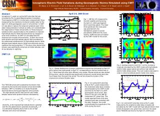
Ionospheric Electric Field Variations during Geomagnetic Storms Simulated using CMIT W. Wang1, A. D. Richmond1, J. Lei1, A. G. Burns1, M. Wiltberger1, S. C. Solomon1, T. L. Killeen1, E. R. Talaat2, and D. L. Hysell3 1High Altitude Observatory, NCAR,2Johns Hopkins University, 3Cornell University LFM Jll, np,Tp E Magnetosphere - Ionosphere Coupler (H+P)=Jll-Jw Particle precipitation: Fe, E0 Conductivities: p, h, Winds: Jw Electric Potential: tot TIE-GCM GSWM April 2-5, 2004 Event Abstract Ionospheric F2 peak ion vertical drift velocities that are simulated by the Coupled Magnetosphere Ionosphere Thermosphere (CMIT) 2.0 model were compared with those measured by the Jicamarca incoherent scatter radar for the April 2-5, 2004 geomagnetic event. It is found that: 1) CMIT 2.0 was able to capture the temporal variations seen in the radar measurements of vertical ion drifts; 2) It overestimated the magnitudes of these vertical drifts; 3) These temporal variations were caused mostly by the variations in imposed high latitude electric fields that were driven by changes in solar wind conditions; 4) CMIT 2.0 simulated well the observed pre-reversal enhancements; 5) Both the neutral wind dynamo and high latitude electric field contributed to the prereversal enhancement; 6) High latitude electric fields affected lower latitude electric fields more efficiently during nighttime that during daytime; 7) The storm-time neutral wind dynamo was significantly enhanced at middle latitudes, and at low latitudes in nighttime. Fig. 1. IMF Bz (nT) measured by the ACE satellite and Kp during the April 2-5, 2004 geomagnetic storm event (top panel). The lower three panels are the cross polar cap potential (kV), the hemispheric power of auroral precipitation (GW) and the Joule heating (GW) that were simulated by the CMIT model for this event. CMIT 2.0 Fig. 4. Eastward electric field (Vm-1) at the Jicamarca longitude simulated by the CMIT model with high latitude electric fields (upper panel) and without high latitude electric fields (lower panel). The color scale is saturated in order to show low latitude electric fields more clearly. Fig. 2. Global distributions of electric potentials at a quiet time (left panel) on April 2nd and a active time (right panel) on April 3rd, corresponding to the two vertical lines in Fig.1. Note these two plots have different color scales. Neutral winds are also plotted. During storm, electric potential was significantly enhanced, neutral winds were also much larger than the quiet time winds. The red dot shows the location of the Jicamarca Incoherent Scatter radar. Fig. 3. Ion vertical drift velocities (m/s) at the F2 peak measured by the Jicamarca radar (blue crosses) and simulated by the CMIT model (red line) for the April 2-5, 2004 geomagnetic storm event. Also shown in the plot is the IMF Bz component (nT, green line). The model captured most of the time variations and was consistent with the data. However, the model overestimated the magnitude of the drifts during the storm. The TIEGCM solves self-consistently the electric field induced by the neutral wind dynamo at low and middle latitudes, CMIT 2.0 enables us to study the global electrodynamics during geomagnetic active periods. The high latitude electric field and low and middle latitude neutral wind dynamo field are calculated by: Fig. 5. Ion vertical drift velocities (m/s) at the F2 peak measured by the Jicamarca radar (blue crosses) and simulated by the CMIT model with high latitude electric field turned off (dynamo only, green line), and from the stand-alone TIEGCM (red line) for the April 2-5, 2004 event. where Φm is the imposed high latitude electric potential and Φ is the global electric potential (including Φm ). P is a latitudinal weighting factor that is zero at high latitudes and one at low latitudes. Center for Integrated Space Weather Modeling • Annual Site Visit • 5 June 2007