Error Diffusion Halftoning Methods for Image Display
Error Diffusion Halftoning Methods for Image Display. Prof. Brian L. Evans. Embedded Signal Processing Laboratory The University of Texas at Austin Austin, TX 78712-1084 USA http:://www.ece.utexas.edu/~bevans.

Error Diffusion Halftoning Methods for Image Display
E N D
Presentation Transcript
Error Diffusion Halftoning Methods forImage Display Prof. Brian L. Evans Embedded Signal Processing Laboratory The University of Texas at Austin Austin, TX 78712-1084 USA http:://www.ece.utexas.edu/~bevans Ph.D. Graduates: Dr. Niranjan Damera-Venkata (HP Labs) Dr. Thomas D. Kite (Audio Precision)Dr. Vishal Monga (Xerox Labs) Ph.D. Student: Mr. Hamood Rehman March 22, 2008
Outline • Introduction • Grayscale error diffusion • Analysis and modeling • Enhancements • Color error diffusion • Vector quantization withseparable filtering • Matrix-valued error filtermethods • Conclusion Barbaraimage Peppersimage
Introduction Need for Digital Image Halftoning • Examples of reduced grayscale/color resolution • Laser and inkjet printers ($9.3B revenue in 2001 in US) • Low-cost liquid crystal displays • Reflective displays, e.g. on cell phones • Halftoning is wordlength reduction for images • Grayscale: 8-bit image to 1-bit image (ink dot, or no ink dot) • Color: 24-bit RGB image to 12-bit RGB display (PDAs) • Halftoning tries to reproduce full range of gray/ color while preserving quality & spatial resolution • Screening methods quantize each pixel value (feedforward) • Error diffusion methods quantize each pixel value and filter resulting quantization error (feedback)
Introduction Need for Speed for Digital Image Halftoning • Third-generation ultra high-speed printer (CMYK) • 100 pages per minute, 600 lines per inch, 4800 dots/inch/line • Output data rate of 7344 MB/s (HDTV video is ~96 MB/s) • Desktop color printer (CMYK) • 24 pages per minute, 600 lines/inch, 600 dots/inch/line • Output data rate of 220 MB/s (NTSC video is ~24 MB/s) • Parallelism in common halftoning algorithms • Screening: pixel-parallel, fast, and easy to implement(2 byte reads, 1 compare, and 1 bit write per binary pixel) • Error diffusion: row-parallel, better results on some media(5 byte reads, 1 compare, 4 MACs, 1 byte and 1 bit write per binary pixel)
Introduction Original Image Threshold at Mid-Gray x(m) b(m) Binarize Image Using a Fixed Threshold • 8-bit grayscale image • Each pixel value represents image intensity • Each pixel value is unsigned 8-bit number in [0, 255] • For display: black is 0, white is 255, and mid-gray is 128 • Threshold each pixel using same fixed threshold • If pixel value 128, output 255; otherwise, output 0
Introduction Screening (Masking) Methods • Periodic thresholds to binarize image • Periodic application leads to aliasing (gridding effect) • Clustered dot screening is more resistant to ink spread • Dispersed dot screening has higher spatial resolution • Blue noise screening uses larger masks (e.g. 1” by 1”) Clustered dot mask Dispersed dot mask index Threshold Lookup Table
Consider 4-bit signal on 2-bit display device Unsigned data Feedback quantization error For constant input of 1001… Average output value 1/4(10+10+10+11) = 1001 4-bit resolution at DC ! Wordlength reduction Truncating 4 bits to 2 bits increases noise by ~12 dB Feedback removes noise at DC but increases noise at high frequency Introduction Inputsignal words 4 2 Todisplaydevice 2 2 Adder Inputs OutputTime Upper Lower Sum to display 1 1001 00 1001 10 2 1001 01 1010 10 3 1001 10 1011 10 4 1001 11 1100 11 1 sample delay added noise 12 dB (2 bits) Periodic f Adding Feedback to Quantization: Example
Introduction Original Image difference threshold current pixel u(m) 7/16 x(m) b(m) _ + 3/16 5/16 1/16 _ + e(m) Error Diffusion compute error shape error error filter weights Error Diffusion Halftoning • Nonlinear feedback system • Quantize each pixel • Filter quantization error (noise) • Add filtered output to “future” grayscale pixels to diffuse quantization error
Introduction Original Image Threshold at Mid-Gray Dispersed Dot Screening Clustered DotScreening Stucki Error Diffusion Floyd SteinbergError Diffusion Conversion to One Bit Per Pixel: Spatial Domain
Introduction Dispersed Dot Screening Threshold at Mid-Gray Original Image Clustered DotScreening Stucki Error Diffusion Floyd SteinbergError Diffusion Conversion to One Bit Per Pixel: Magnitude Spectra
Introduction Human Visual System Modeling • Contrast at particular spatialfrequency for visibility • Bandpass: non-dimbackgrounds[Manos & Sakrison, 1974; 1978] • Lowpass: high-luminance officesettings with low-contrast images[Georgeson & G. Sullivan, 1975] • Exponential decay[Näsäsen, 1984] • Modified lowpass version[e.g. J. Sullivan, Ray & Miller, 1990] • Angular dependence: cosinefunction[Sullivan, Miller & Pios, 1993]
Introduction Error Diffusion difference threshold current pixel u(m) 7/16 x(m) b(m) _ + 3/16 5/16 1/16 _ + e(m) compute error Spectrum shape error error filter weights Grayscale Error Diffusion Halftoning • Aperiodic halftones • Shape quantization noise into highfrequencies, which are less visible • Design of error filter key to quality
Analysis and Modeling Raster Serpentine Analysis of Error Diffusion I • Error diffusion as 2-D sigma-delta modulation[Anastassiou, 1989] [Bernard, 1991] • Error image[Knox, 1992] • Error image correlated with input image • Sharpening proportional to correlation • Serpentine scan places morequantization error along diagonalfrequencies than raster [Knox, 1993] • Threshold modulation[Knox, 1993] • Add signal (e.g. white noise) to quantizer input • Equivalent to error diffusing an input image modified by threshold modulation signal
Analysis and Modeling Example: Role of Error Image • Sharpening proportional to correlation between error image and input image[Knox, 1992] Floyd-Steinberg(1976) Limit Cycles Jarvis(1976) Error images Halftones
Analysis and Modeling Analysis of Error Diffusion II • Limit cycle behavior[Fan & Eschbach, 1993] • For a limit cycle pattern, quantified likelihood of occurrence for given constant input as function of filter weights • Reduced likelihood of limit cycle patterns by changing filter weights • Stability of error diffusion[Fan, 1993] • Sufficient conditions for bounded-input bounded-error stability: sum of absolute values of filter coefficients is one • Green noise error diffusion[Levien, 1993] [Lau, Arce & Gallagher, 1998] • Promotes minority dot clustering • Linear gain model for quantizer[Kite, Evans & Bovik, 2000] • Models sharpening and noise shaping effects (next slide) Minority pixels
Analysis and Modeling Q(x) 255 x { 0 us(m) Ks us(m) 0 128 255 Ks Signal Path u(m) b(m) Q(.) n(m) un(m) + n(m) un(m) Noise Path Linear Gain Model for Quantizer • Sigma-delta modulation analysis Linear gain model for quantizer in 1-D[Ardalan and Paulos, 1988] Linear gain model for grayscale image[Kite, Evans, Bovik, 1997] • Models error diffusion as linear, shift-invariant Signal transfer function (STF): quantizer acts as scalar gain Noise transfer function (NTF): quantizer acts as additive noise
Analysis and Modeling Linear Gain Model for Quantizer n(m) Quantizermodel x(m) u(m) b(m) Ks _ + f(m) _ • Put noise in high frequencies • H(z) must be lowpass + e(m) STF NTF 2 1 1 w w w -w1 -w1 -w1 w1 w1 w1 Also, let Ks = 2 (Floyd-Steinberg) Pass low frequencies Enhance high frequencies Highpass response(independent of Ks )
Image Floyd Stucki Jarvis Analysis and Modeling barbara 2.01 3.62 3.76 boats 1.98 4.28 4.93 lena 2.09 4.49 5.32 mandrill 2.03 3.38 3.45 Average 2.03 3.94 4.37 Linear Gain Model for Quantizer • Best linear fit for Ks between quantizer input u(m) and halftone b(m) • Does not vary much for Floyd-Steinberg • Can use average value to estimate Ks from only error filter • Sharpening: proportional to Ks [Kite, Evans & Bovik, 2000] Value of Ks: Floyd Steinberg < Stucki < Jarvis • Weighted SNR using unsharpened halftone Floyd-Steinberg > Stucki > Jarvis at all viewing distances
Enhancements Enhancements I: Error Filter Design • Longer error filters reduce directional artifacts[Jarvis, Judice & Ninke, 1976] [Stucki, 1981] [Shiau & Fan, 1996] • Fixed error filter design: minimize mean-squared error weighted by a contrast sensitivity function Assume error image is white noise [Kolpatzik & Bouman, 1992] Off-line training on images [Wong & Allebach, 1998] • Adaptive least squares error filter[Wong, 1996] • Tone dependent filter weights for each gray level [Eschbach, 1993] [Shu, 1995] [Ostromoukhov, 1998] [Li & Allebach, 2002]
Enhancements Tone dependent threshold modulation b(m) x(m) _ + _ + Tone dependent error filter Midtone regions e(m) FFT DBS pattern for graylevel x Halftone pattern for graylevel x FFT Example: Tone Dependent Error Diffusion • Train error diffusionweights and thresholdvalue for each inputgray level [Li & Allebach, 2002] Highlights and shadows FFT Graylevel patch x Halftone pattern for graylevel x FFT
Enhancements Enhancements II: Controlling Artifacts • Sharpness control • Edge enhancement error diffusion[Eschbach & Knox, 1991] • Linear frequency distortion removal[Kite, Evans & Bovik, 1999] • Adaptive linear frequency distortion removal[Damera-Venkata & Evans, 2001] • Reducing worms in highlights & shadows[Eschbach, 1993] [Shu, 1993] [Levien, 1993] [Eschbach, 1996] [Marcu, 1998] • Reducing mid-tone artifacts • Filter weight perturbation[Ulichney, 1988] • Threshold modulation with noise array[Knox, 1993] • Deterministic bit flipping quant. [Damera-Venkata & Evans, 2001] • Tone dependent modification[Li & Allebach, 2002] DBF(x) x
Enhancements Example: Sharpness Control in Error Diffusion • Adjust by threshold modulation [Eschbach & Knox, 1991] • Scale image by gain L and add it to quantizer input • Low complexity: one multiplication, one addition per pixel • Flatten signal transfer function [Kite, Evans & Bovik, 1999] L b(m) u(m) x(m) _ + _ + e(m)
Enhancements Original Floyd-Steinberg Results Edge enhanced Unsharpened
Enhancements Enhancements III: Clustered Dot Error Diffusion • Feedback output to quantizer input [Levien, 1993] • Dot to dot error diffusion [Fan, 1993] • Apply clustered dot screen on block and diffuse error • Reduces contouring • Clustered minority pixel diffusion [Li & Allebach, 2000] • Block error diffusion [Damera-Venkata & Evans, 2001] • Clustered dot error diffusion using laser pulse width modulation [He & Bouman, 2002] • Simultaneous optimization of dot density and dot size • Minimize distortion based on tone reproduction curve
Enhancements Block error diffusion Green-noise Results DBF quantizer Tone dependent
Color Error Diffusion YUV to RGB Conversion Color Monitor Display Example (Palettization) • YUV color space • Luminance (Y) and chrominance (U,V) channels • Widely used in video compression standards • Contrast sensitivity functions available for Y, U, and V • Display YUV on lower-resolution RGB monitor: use error diffusion on Y, U, V channels separably u(m) b(m) 24-bit YUV video 12-bit RGB monitor x(m) + _ _ + RGB to YUV Conversion h(m) e(m)
Color Error Diffusion Non-Separable Color Halftoning for Display • Input image has a vector of values at each pixel (e.g. vector of red, green, and blue components) Error filter has matrix-valued coefficients Algorithm for adaptingmatrix coefficientsbased on mean-squarederror in RGB space[Akarun, Yardimci & Cetin, 1997] • Optimization problem Given a human visual system model, findcolor error filter that minimizes average visible noise power subject to diffusion constraints [Damera-Venkata & Evans, 2001] Linearize color vector error diffusion, and use linear vision model in which Euclidean distance has perceptual meaning u(m) x(m) b(m) _ + _ t(m) e(m) +
Color Error Diffusion Matrix Gain Model for the Quantizer • Replace scalar gain w/ matrix [Damera-Venkata & Evans, 2001] • Noise uncorrelated with signal component of quantizer input • Convolution becomes matrix–vector multiplication in frequency domain u(m) quantizer inputb(m) quantizer output Grayscale results Noisecomponentof output Signalcomponentof output
Color Error Diffusion Linear Color Vision Model • Undo gamma correction to map to sRGB • Pattern-color separable model [Poirson & Wandell, 1993] • Forms the basis for Spatial CIELab [Zhang & Wandell, 1996] • Pixel-based color transformation B-W R-G B-Y Spatial filtering Opponent representation
Color Error Diffusion Example Original SeparableFloyd-Steinberg Optimum vectorerror filter
Color Error Diffusion Evaluating Linear Vision Models[Monga, Geisler & Evans, 2003] • Objective measure: improvement in noise shaping over separable Floyd-Steinberg • Subjective testing based on paired comparison task Online at www.ece.utexas.edu/~vishal/cgi-bin/test.html • In decreasing subjective (and objective) quality Linearized CIELab > > Opponent > YUV YIQ original halftone A halftone B
Grayscale andcolor methods Screening Classical diffusion Edge enhanced diff. Green noise diffusion Block diffusion Figures of merit Peak SNR Weighted SNR Linear distortion measure Universal quality index Conclusion Image Halftoning Toolbox 1.2 Figures of Merit http://www.ece.utexas.edu/~bevans/projects/halftoning/toolbox
Introduction Q[x] 1 x -2 1 -2 Uniform Quantization Using Thresholding • Round to nearest integer (midtread) Quantize amplitude to levels {-2, -1, 0, 1} Step size D for linear region of operation Represent levels by {00, 01, 10, 11} or{10, 11, 00, 01} … Latter is two's complement representation • Rounding with offset (midrise) Quantize to levels {-3/2, -1/2, 1/2, 3/2} Represent levels by {11, 10, 00, 01} … Step size Q[x] 1 x -2 1 2 -1
Introduction current pixel Floyd-Steinbergweights 7/16 3/16 5/16 1/16 x(m) b(m) _ + _ + shape error e(m) Error Diffusion Original Halftone u(m)
Introduction Digital Halftoning Methods Clustered Dot Screening AM Halftoning Dispersed Dot Screening FM Halftoning Error Diffusion FM Halftoning 1976 Blue-noise MaskFM Halftoning 1993 Green-noise Halftoning AM-FM Halftoning 1992 Direct Binary Search FM Halftoning 1992
Analysis and Modeling Compensation for Frequency Distortion • Flatten signal transfer function [Kite, Evans, Bovik, 2000] • Pre-filtering equivalent to threshold modulation x(m) u(m) g(m) b(m) _ + _ + e(m)
Analysis and Modeling Visual Quality Measures [Kite, Evans & Bovik, 2000] • Sharpening: proportional to Ks Value of Ks: Floyd Steinberg < Stucki < Jarvis • Impact of noise on human visual system Signal-to-noise (SNR) measures appropriate when noise is additive and signal independent Create unsharpened halftone y[m1,m2] with flat signal transfer function using threshold modulation Weight signal/noise by contrast sensitivity function C[k1,k2] Floyd-Steinberg > Stucki > Jarvis at all viewing distances
Enhancements Example #1: Green Noise Error Diffusion • Output fed back to quantizer input [Levien, 1993] • Gain G controls coarseness of dot clusters • Hysteresis filter f affects dot cluster shape f G u(m) b(m) x(m) _ + _ + e(m)
Enhancements difference threshold u(m) x(m) b(m) _ + t(m) _ + e(m) 7/16 shape error compute error 3/16 5/16 1/16 Example #2: Block Error Diffusion • Process a pixel-block using a multifilter[Damera-Venkata & Evans, 2001] • FM nature controlled by scalar filter prototype • Diffusion matrix decides distribution of error in block • In-block diffusions constant for all blocks to preserve isotropy
Enhancements diffusion matrix 7/16 3/16 5/16 1/16 is the block size Block FM Halftoning Error Filter Design • FM nature of algorithm controlled by scalar filter prototype • Diffusion matrix decides distribution of error within a block • In-block diffusions are constant for all blocks to preserve isotropy
Color Error Diffusion MBVC Allowable colors u(m) b(m) VQ x(m) _ + _ + e(m) Vector Quantization but Separable Filtering • Minimum Brightness Variation Criterion(MBVC)[Shaked, Arad, Fitzhugh & Sobel, 1996] • Limit number of output colors to reduce luminance variation • Efficient tree-based quantization to render best color among allowable colors • Diffuse errors separably
Color Error Diffusion Results Original SeparableFloyd-Steinberg MBVC halftone
Color Error Diffusion Linear Color Vision Model • Undo gamma correction on RGB image • Color separation [Damera-Venkata & Evans, 2001] • Measure power spectral distribution of RGB phosphor excitations • Measure absorption rates of long, medium, short (LMS) cones • Device dependent transformation C from RGB to LMS space • Transform LMS to opponent representation using O • Color separation may be expressed as T = OC • Spatial filtering included using matrix filter • Linear color vision model is a diagonal matrix where
Color Error Diffusion linear model of human visual system matrix-valued convolution Designing the Error Filter • Eliminate linear distortion filtering before error diffusion • Optimize error filter h(m) for noise shaping Subject to diffusion constraints where
Color Error Diffusion Generalized Optimum Solution • Differentiate scalar objective function for visual noise shaping w/r to matrix-valued coefficients • Write norm as trace and differentiate trace usingidentities from linear algebra
Color Error Diffusion Generalized Optimum Solution (cont.) • Differentiating and using linearity of expectation operator give a generalization of the Yule-Walker equations where • Assuming white noise injection • Solve using gradient descent with projection onto constraint set
Color Error Diffusion Implementation of Vector Color Error Diffusion Hgr Hgg + Hgb
Color Error Diffusion C1 C2 C3 Representation inarbitrary color space Spatial filtering Generalized Linear Color Vision Model • Separate image into channels/visual pathways • Pixel based linear transformation of RGB into color space • Spatial filtering based on HVS characteristics & color space • Best color space/HVS model for vector error diffusion? [Monga, Geisler & Evans 2002]
Color Error Diffusion Linear CIELab Space Transformation[Flohr, Kolpatzik, R.Balasubramanian, Carrara, Bouman, Allebach, 1993] • Linearized CIELab using HVS Model by Yy = 116 Y/Yn – 116 L = 116 f (Y/Yn) – 116 Cx = 200[X/Xn – Y/Yn] a = 200[ f(X/Xn ) – f(Y/Yn ) ] Cz = 500 [Y/Yn – Z/Zn] b = 500 [ f(Y/Yn ) – f(Z/Zn ) ] where f(x) = 7.787x + 16/116 0<= x <= 0.008856 f(x) = (x)1/3 0.008856 <= x <= 1 • Linearize the CIELab Color Space about D65 white point Decouples incremental changes in Yy, Cx, Cz at white point on (L,a,b) values T is sRGB CIEXYZ Linearized CIELab