Definition of Economics

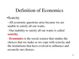
1. Definition of Economics • Scarcity • All economic questions arise because we are unable to satisfy all our wants. • Our inability to satisfy all our wants is called scarcity. • Economics is the social science that studies the choices that we make as we cope with scarcity and the institutions that have evolved to influence and reconcile our choices. 1-1

2. Definition: Economics • Economics is the study of how individuals and societies choose to use the scarce resources that nature and previous generations have provided. • Economics is the study of how scarce resources are allocated among conflicting demands.

3. The Scope of Economics • Microeconomics • Microeconomics is the study of choices made by individuals and businesses, the way these choices interact, and the influence that governments exert on them. • Macroeconomics • Macroeconomics is the study of the effects on the national and global economy of the choices that individuals, businesses, and governments make. 1-3

4. The Scope of Economics

5. Opportunity Costs • The opportunity cost of something is that which we give up when we make that choice or decision. • The implication is that all decisions involve trade-offs. • “There’s no such thing as a free lunch!!”

6. Margins and Incentives • People make choices at themargin, which means that they evaluate the consequences of making incremental changes in the use of their resources. • The benefit from pursuing an incremental increase in an activity is its marginal benefit. • The opportunity cost of pursuing an incremental increase in an activity is its marginal cost. 1-6

7. The Theory of Comparative Advantage • Ricardo’s theory that specialization and free trade will benefit all trading parties, even those that may be absolutely more efficient producers. • A person or country is said to have a comparative advantage in producing a good if it is relatively more efficient than a trading partner at doing so. In other words they have a lower opportunity cost.

8. Production Possibilities andOpportunity Cost • The production possibilities frontier (PPF) is the boundary between those combinations of goods and services that can be produced and those that cannot. • To illustrate the PPF, we focus on two goods at a time and hold the quantities of all other goods and services constant. • That is, we look at a model economy in which everything remains the same (ceteris paribus) except the two goods we’re considering. 2-8

9. Production Possibilities andOpportunity Cost • Production Efficiency • We achieve production efficiency if we cannot produce more of one good without producing less of some other good. • Points on the frontier are efficient. 2-9

10. Production Possibilities andOpportunity Cost • A move from C to D increases butter production by 1 tonne. • Guns production decreases from 12 units to 9 units, a decrease of 3 units. • The opportunity cost of 1 tonne of butter is 3 units of guns. • One tonne of butter costs 3 units of guns. 2-10

11. Using Resources Efficiently • All the points along the PPF are efficient. • To determine which of the alternative efficient quantities to produce, we compare costs and benefits. • The PPF and Marginal Cost • The PPF determines opportunity cost. • The marginal cost of a good or service is the opportunity cost of producing one more unit of it. 2-11

12. Using Resources Efficiently • Preferences and Marginal Benefit • Preferences are a description of a person’s likes and dislikes. • To describe preferences, economists use the concepts of marginal benefit and the marginal benefit curve. • The marginal benefit of a good or service is the benefit received from consuming one more unit of it. • We measure marginal benefit by the amount that a person is willing to pay for an additional unit of a good or service. • It is a general principle that the more we have of any good or service, the smaller its marginal benefit and the less we are willing to pay for an additional unit of it. • We call this general principle the principle of decreasing marginal benefit. 2-12

13. When we cannot produce more of any one good without giving up some other good that we value more highly, we have achieved allocative efficiency, and we are producing at the point on the PPF that we prefer above all other points. • The point of allocative efficiency is the point on the PPF at which marginal benefit equals marginal cost.

14. Determinants of Household Demand: • The price of the product in question • The income available to the household • The households amount of accumulated wealth • The prices of other products available • Tastes and preferences • Expectations about future income, wealth, and prices • Population

15. Changes in Quantity Demanded vs. Changes in Demand • Changes in the price of a product affect the quantity demanded per period. Changes in any other factor, such as income or preferences, affect demand. An increase in income, for instance, tends to increase demand. While a drop in prices will increase the quantity demanded.

16. The Law of Demand • The negative relationship between price and quantity demanded. As price rises, quantity demanded decreases. As price falls, quantity demanded increases • This is why we observe a negative slope in demand curves.

17. Substitution EffectWhen the relative price (opportunity cost) of a good or service rises, people seek substitutes for it, so the quantity demanded decreases.When the price of a product falls, that product becomes more attractive relative to potential substitutes.Income EffectWhen the price of a good or service rises relative to income, people cannot afford all the things they previously bought, so the quantity demanded decreases.When the price of a product falls, a consumer has more purchasing power with the same amount of income and is better off.

18. Income as a Determinant of Demand Income: The total of all earnings received by a household in a given period of time • Normal Goods: Goods for which demand goes up when income is higher and for which demand goes down when income is lower. • Inferior Goods: Goods for which demand falls when income rises.

19. Prices of Other Goods and Services as Determinants ofDemand • Substitutes: Goods that can serve as replacements for one another; when the price of one increases, demand for the other goes up. • Perfect substitutes are identical products. • Complements: Goods that “go together”; when the price of one increases, demand for the other goes down, and vice versa.

20. Other Determinants of Household Demand: • Tastes and Preferences - These are quite subjective and tend to change over time. • Expectations - With respect to future income, wealth, prices, and availability.

21. Shift of Demand vs. Movement Along Demand Curve • Shift of a demand curve is the change that takes place in a demand curve when a new relationship between the quantity demanded of a good and the price of that good is brought about by a change in the original conditions. • Movement along the demand curve is what happens when a change in price causes quantity demanded to change.

22. Price $15.00 $10.00 $7.50 $3.50 $ .50 0 1 3 7 25 30 Quantity demanded Anna’s Demand for Telephone Calls -A Change in Quantity Demanded • The graph shows a shift in quantity demanded from 3 to 7 caused by a change in price from $7.50 to $3.50.

23. D2 D1 25 30 Anna’s Demand for Telephone Calls - A Change in Demand • When any factor except price changes the relationship between price and quantity is different; there is a shift of the demand curve, in this case from D1 to D2. $15.00 $10.00 $7.50 $3.50 $ .50 0 1 3 7

24. Changes in Demand: Prices of Related Goods P Price of hamburger rises P P Q Quantity of hamburger demanded falls D1 D2 D2 D1 Demand for complement good (ketchup) shifts left Q Demand for substitute good (chicken) shifts right Q

25. From Household to Market Demand • Demand for a good or service can be defined for an individual household, or for a group of households that make up a market. • Market demand may be defined as the sum of all the quantities of a good or service demanded per period by all the households buying in the market for that good or service.

26. Deriving market demand from the individual demand curves: P P P $3.50 DA $3.50 DC DB $3.50 $1.50 $1.50 $1.50 0 0 0 3 Qd 4 8 Qd 4 9 Qd Price Market Demand $3.50 $1.50 0 8 20 Qd

27. Supply • A firm’s decision about what quantity of product to supply depends on: • The price of the good or service • The cost of producing the product which depends on: • The price of required inputs (land, labour, capital) • The technologies to be used to produce the product • The prices of related products • Expected future prices • The number of suppliers

28. Quantity Supplied andThe Law of Supply • Quantity Supplied : The amount of a particular product that a firm would be willing and able to offer for sale at a particular price during a given time period. • The Law of Supply : The positive relationship between price and quantity of a good supplied. An increase in market price will lead to an increase in quantity supplied, and a decrease in market price will lead to a decrease in quantity supplied.

29. Changes in Quantity Supplied vs.Changes in Supply: Changes in quantity supplied imply movement along a supply curve.Changes in supply imply a shift in the entire supply curve. P P S S1 S2 Q Q An increase in supply An increase in the quantity supplied

30. From Individual Firm to Market Supply: Market Supply • The supply of a good or service can be defined for an individual firm, or for a group of firms that make up a market or an industry. • Market Supply : The sum of all the quantities of a good or service supplied per period by all the firms selling in the market for that good or service. • As with market demand, market supply is the horizontal summation of the individual firms’ supply curves.

31. From Individual Firm to Market Supply

32. Market Equilibrium • The operation of the market depends on the interaction between suppliers and demanders. • An equilibrium is the condition that exists when quantity supplied and quantity demanded are equal. • At equilibrium, there is no tendency for the price to change.

33. Market Equilibrium P S E PE D Q QE

34. Excess Demand: is the condition that exists when quantity demanded exceeds quantity supplied at the current price. • At $85 per tonne quantity demanded exceeds quantity supplied by 2500 tonnes. • Excess demand tends to lead to an increase in prices.

35. Excess Supply: Excess supply is the condition that exists when quantity supplied exceeds quantity demanded at the current price. • At $150, quantity supplied exceeds the quantity demanded by 2000 tonnes. • This causes prices to fall

36. Price Elasticity of Demand • The price elasticity of demand is the ratio of the percentage change in quantity demanded to the percentage change in price. • Price Elasticity of Demand = % change in quantity demanded % change in price

37. Inelastic Demand • Perfectly inelastic demand is demand in which quantity demanded does not respond at all to a change in price. • An example could be the demand for insulin. • Inelastic demand is demand that responds somewhat, but not a great deal, to changes in price. Inelastic demand always has a numerical value between zero minus one. • An example would be the demand for housing or telephone service.

38. Unitary Elasticity • Unitary elasticity is a demand relationship in which the percentage change in quantity of a product demanded is the same as the percentage change in price. • The elasticity is always equal to minus one.

39. Elastic Demand • Elastic demand is a demand relationship in which the percentage change in quantity demanded is larger in absolute value than the percentage change in price. • The demand elasticity has an absolute value greater than one. • An example could be the demand for bananas or any other product for which there are close substitutes. • Perfectly elastic demand is demand in which quantity demanded drops to zero at the slightest increase in price. • An example could be the demand for wheat on the world market, or any other good that can only be sold at a predetermined price.

40. Demand Curves and Elasticity P P D D Q Q Perfectly elastic Relatively elastic D P P D Q Q Perfectly inelastic Relatively inelastic

41. Elasticity and Total Revenue • Effect of a price increase on a product with inelastic demand: P x Qd = TR • Effect of a price increase on a product with elastic demand: P x Qd = TR • Effect of a price cut on a product with elastic demand: P x Qd = TR • Effect of price cut on a product with inelastic demand: P x Qd = TR

42. Relationship Between Elasticity and Total Revenue

43. Determinants of Demand Elasticity • Availability of substitutes • When substitutes are not readily available, demand is likely to be less elastic. • The importance of being unimportant • When an item represents a small proportion of our total budget, demand is likely to be less elastic. • The time dimension • In the longer run, demand is likely to become more elastic, or responsive, because households make adjustments over time.

44. Other Important Elasticities • Income elasticity of demand • Measures the responsiveness of demand with respect to changes in income • If the income elasticity of demand is greater than 1, demand is income elastic and the good is a normal good. • If the income elasticity of demand is greater than zero but less than 1, demand is income inelastic and the good is a normal good. • If the income elasticity of demand is less than zero (negative) the good is an inferior good. • Cross-price elasticity of demand • A measure of the response of the quantity of one good demanded to a change in the price of another good • The cross elasticity of demand for a substitute is positive. • The cross elasticity of demand for a complement is negative. • Elasticity of supply • A measure of the response of the quantity of a good supplied to a change in the price of that good. Likely to be positive in output markets

45. Efficiency: A Refresher • An efficient allocation of resources occurs when we produce the goods and services that people value most highly. • Resources are allocated efficiently when it is not possible to produce more of a good or service without giving up some other good or service that is valued more highly. 5-45

46. Value, Willingness to Pay, and Demand • The value of one more unit of a good or service is its marginal benefit, which we can measure as maximum price that a person is willing to pay. • A demand curve for a good or service shows the quantity demanded at each price. • A demand curve also shows the maximum price that consumers are willing to pay at each quantity. 5-46

47. Cost, Minimum Supply-Price, and Supply • The cost of one more unit of a good or service is its marginal cost, which we can measure as minimum price that a firm is willing to accept. • A supply curve of a good or service shows the quantity supplied at each price. A supply curve also shows the minimum price that producers are willing to accept at each quantity. 5-47

48. Producer Surplus, Consumer surplus • Producer surplus is the price of a good minus the marginal cost of producing it, summed over the quantity sold. • Producer surplus is measured by the area below the price and above the supply curve, up to the quantity sold. • Consumer surplus is the value of a good minus the price paid for it, summed over the quantity bought. • It is measured by the area under the demand curve and above the price paid, up to thequantity bought. 5-48

49. Is the Competitive Market Efficient? • At the equilibrium quantity, marginal benefit equals marginal cost, so the quantity is the efficient quantity. • The sum of consumer and producer surplus is maximized at this efficient level of output. 5-49

50. Is the Competitive Market Efficient? • Obstacles to Efficiency • Markets are not always efficient. Obstacles to efficiency are: • Price ceilings and floors • Taxes, subsidies, and quotas • Monopoly • Public goods • External costs and external benefits 5-50