Download
1 / 49
490 likes | 691 Vues
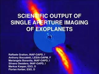
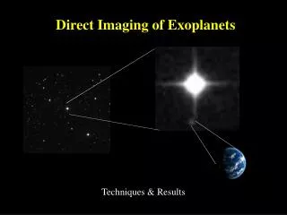
Direct Imaging of Exoplanets. Techniques & Results. Challenge 1: Large ratio between star and planet flux (Star/Planet). Reflected light from Jupiter ≈ 10 –9. Stars are a billion times brighter…. …than the planet. …hidden in the glare.

E N D
Direct Imaging of Exoplanets Techniques & Results
Challenge 1: Large ratio between star and planet flux (Star/Planet) Reflected light from Jupiter ≈ 10–9
…than the planet …hidden in the glare.
Challenge 2: Close proximity of planet to host star Direct Detections need contrast ratios of 10–9 to 10–10 At separations of 0.01 to 1 arcseconds Earth : ~10–10 separation = 0.1 arcseconds for a star at 10 parsecs Jupiter: ~10–9 separation= 0.5 arcseconds for a star at 10 parsecs 1 AU = 1 arcsec separation at 1 parsec
Younger planets are hotter and they emit more radiated light. These are easier to detect.
Adaptive Optics : An important component for any imaging instrument Atmospheric turbulence distorts stellar images making them much larger than point sources. This seeing image makes it impossible to detect nearby faint companions.
Adaptive Optics (AO) The scientific and engineering discipline whereby the performance of an optical signal is improved by using information about the environment through which it passes AO Deals with the control of light in a real time closed loop and is a subset of active optics. Adaptive Optics: Systems operating below 1/10 Hz Active Optics: Systems operating above 1/10 Hz
Example of an Adaptive Optics System: The Eye-Brain The brain interprets an image, determines its correction, and applies the correction either voluntarily of involuntarily Lens compression: Focus corrected mode Tracking an Object: Tilt mode optics system Iris opening and closing to intensity levels: Intensity control mode Eyes squinting: An aperture stop, spatial filter, and phase controlling mechanism
The Ideal Telescope image of a star produced by ideal telescope • where: • P(a) is the light intensity in the focal plane, as a function of angular coordinates a ; • l is the wavelength of light; • D is the diameter of the telescope aperture; • J1 is the so-called Bessel function. • The first dark ring is at an angular distance Dl of from the center. • This is often taken as a measure of resolution (diffraction limit) in an ideal telescope. Dl = 1.22 l/D = 251643 l/D (arcsecs)
Diffraction Limit Telescope 5500 Å 2 mm 10 mm Seeing TLS 2m 0.06“ 0.2“ 1.0“ 2“ 0.06“ 0.3“ 0.017“ 0.2“ VLT 8m Keck 10m 0.014“ 0.05“ 0.25“ 0.2“ 0.1“ 0.2“ ELT 42m 0.003“ 0.01“ Even at the best sites AO is needed to improve image quality and reach the diffraction limit of the telescope. This is easier to do in the infrared
Atmospheric Turbulence Original wavefront • Turbulence causes temperature fluctuations • Temperature fluctuations cause refractive index variations • Turbulent eddies are like lenses • Plane wavefronts are wrinkled and star images are blurred Distorted wavefront
Basic Components for an AO System • You need to have a mathematical model representation of the wavefront • You need to measure the incoming wavefront with a point source (real or artifical). • You need to correct the wavefront using a deformable mirror
Shack-Hartmann Wavefront Sensor Lenslet array Image Pattern reference Focal Plane detector af disturbed a f
If you are observing an object here You do not want to correct using a reference star in this direction
Reference Stars You need a reference point source (star) for the wavefront measurement. The reference star must be within the isoplanatic angle, of about 10-30 arcseconds If there is no bright (mag ~ 14-15) nearby star then you must use an artificial star or „laser guide star“. All laser guide AO systems use a sodium laser tuned to Na 5890 Å pointed to the 11.5 km thick layer of enhanced sodium at an altitude of 90 km. Much of this research was done by the U.S. Air Force and was declassified in the early 1990s.
Applications of Adaptive Optics Sun, planets, stellar envelopes and dusty disks, young stellar objects, galaxies, etc. Can get 1/20 arcsecond resolution in the K band, 1/100 in the visible (eventually)
Applications of Adaptive Optics • Faint companions • The seeing disk will normally destroy the image of faint companion. Is needed to detect substellar companions (e.g. GQ Lupi)
Applications of Adaptive Optics • Coronagraphy • With a smaller image you can better block the light. Needed for planet detection
Subtracting the Point Spread Function (PSF) To detect close companions one has to subtract the PSF of the central star (even with coronagraphs) which is complicated by atmospheric speckles. One solution: Differential Imaging
Nulling Interferometers Adjusts the optical path length so that the wavefronts from both telescope destructively interfere at the position of the star Technological challenges have prevented nulling interferometry from being a viable imaging method…for now
Darwin/Terrestrial Path Finder would have used Nulling Interferometry Earth Venus Mars Ground-based European Nulling Interferometer Experiment will test nulling interferometry on the VLTI
Coronography of Debris Disks Structure in the disks give hints to the presence of sub-stellar companions
Another brown dwarf detected with the NACO adaptive optics system on the VLT
The Planet Candidate around GQ Lupi But there is large uncertainty in the surface gravity and mass can be as low as 4 and as high as 155 MJup depending on which evolutionary models are used.
a ~ 115 AU P ~ 870 years Mass < 3 MJup, any more and the gravitation of the planet would disrupt the dust ring
Photometry of Fomalhaut b Planet model with T = 400 K and R = 1.2 RJup. Reflected light from circumplanetary disk with R = 20 RJup Detection of the planet in the optical may be due to a disk around the planet. Possible since the star is only 30 Million years old.
using Angular Differential Imaging (ADI):
The Planet around b Pic Mass ~ 8 MJup
2003 2009
Imaging Planet Candidates 1SIMBAD lists this as an A5 V star, but it is a g Dor variable which have spectral types F0-F2. Spectra confirm that it is F-type 2A fourth planet around HR 8799 was reported at the 2011 meeting of the American Astronomical Society
Summary of Direct Imaging: • Most challenging observational technique due to proximity, contrast levels and atmospheric effects (AO, coronagraphy,..) • Candidates appeared at large (~100 AU) separations and mass determination is limited by reliability of evolutionary models (if no other information) • More robust detections (3) include a multi-planet system (HR 8799) and two planets around stars with a large debris disk (Fomalhaut, beta Pic) • Massive planets around massive stars (A,F-type) at large separations (no Solar System analogues yet) different class of exoplanets?