Download
1 / 95
970 likes | 1.19k Vues
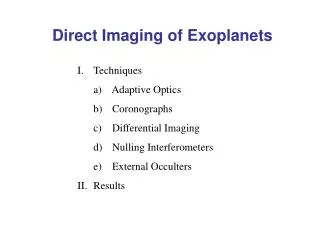
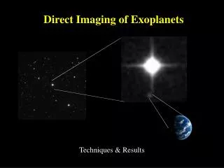
Techniques Adaptive Optics Coronographs Differential Imaging Results. Direct Imaging of Exoplanets. Challenge 1: Large ratio between star and planet flux (Star/Planet). Reflected light from Jupiter ≈ 10 –9. Challenge 2: Close proximity of planet to host star.

E N D
Techniques • Adaptive Optics • Coronographs • Differential Imaging • Results Direct Imaging of Exoplanets
Challenge 1: Large ratio between star and planet flux (Star/Planet) Reflected light from Jupiter ≈ 10–9
Challenge 2: Close proximity of planet to host star Direct Detections need contrast ratios of 10–9 to 10–10 At separations of 0.01 to 1 arcseconds Earth : ~10–10 separation = 0.1 arcseconds for a star at 10 parsecs Jupiter: ~10–9 separation= 0.5 arcseconds for a star at 10 parsecs 1 AU = 1 arcsec separation at 1 parsec
Younger planets are hotter and they emit more radiated light. These are easier to detect.
A Little Background: Fourier Transforms f(x) = F(s) e2pixs ds F(s) = f(x) e−2pixs dx The Fourier transform of a function (frequency spectrum) tells you the amplitude (contribution) of each sin (cos) function at the frequency that is in the function under consideration. The square of the Fourier transform is the power spectra and is related to the intensity when dealing with light.
Fourier Transforms Two important features of Fourier transforms: 1) The “spatial or time coordinate” x maps into a “frequency” coordinate 1/x (= s or n) Thus small changes in x map into large changes in s. A function that is narrow in x is wide in s
A Pictoral Catalog of Fourier Transforms Time/Space Domain Fourier/Frequency Domain 0 Time Frequency (1/time) Period = 1/frequency Comb of Shah function (sampling function) x 1/x
Time/Space Domain Fourier/Frequency Domain Negative frequencies Positive frequencies Cosine is an even function: cos(–x) = cos(x)
Time/Space Domain Fourier/Frequency Domain Sine is an odd function: sin(–x) = –sin(x)
Time/Space Domain Fourier/Frequency Domain e–px2 e–ps2 w 1/w The Fourier Transform of a Gausssian is another Gaussian. If the Gaussian is wide (narrow) in the temporal/spatial domain, it is narrow(wide) in the Fourier/frequency domain. In the limit of an infinitely narrow Gaussian (d-function) the Fourier transform is infinitely wide (constant)
Time/Space Domain Fourier/Frequency Domain All functions are interchangeable. If it is a sinc function in time, it is a slit function in frequency space Note: these are the diffraction patterns of a slit, triangular and circular apertures
Fourier Transforms : Convolution Convolution f(u)f(x–u)du = f * f f(x): f(x):
f(x-u) a2 a3 a1 a2 a3 a1 Cross Correlation g(x) CCF
x Background: Fourier Transforms In Fourier space the convolution (smoothing of a function) is just the product of the two transforms: Normal Space Fourier Space f*g F G Suppose you wanted to smooth your data by n points. • You can either: • Move your box to a place in your data, average all the points in that box for value 1, then slide the box to point two, average all points in box and continue. • Compute FT of data, the FT of box function, multiply the two and inverse Fourier transform
sinc sinc2 Fourier Transforms The second important features of Fourier transforms: 2) In Fourier space the convolution is just the product of the two transforms: Normal Space Fourier Space f*g F G f g F * G
Adaptive Optics : An important component for any coronagraph instrument Seeing → 0.5“ 1“ 0.25“ 2“ Atmospheric turbulence distorts stellar images making them much larger than point sources. This seeing image makes it impossible to detect nearby faint companions.
Adaptive Optics The scientific and engineering discipline whereby the performance of an optical signal is improved by using information about the environment through which it passes AO Deals with the control of light in a real time closed loop and is a subset of active optics. Adaptive Optics: Systems operating below 1/10 Hz Active Optics: Systems operating above 1/10 Hz
Example of an Adaptive Optics System: The Eye-Brain The brain interprets an image, determines its correction, and applies the correction either voluntarily of involuntarily Lens compression: Focus corrected mode Tracking an Object: Tilt mode optics system Iris opening and closing to intensity levels: Intensity control mode Eyes squinting: An aperture stop, spatial filter, and phase controlling mechanism
The Ideal Telescope This is the Fourier transform of the telescope aperture • where: • P(a) is the light intensity in the focal plane, as a function of angular coordinates a ; • l is the wavelength of light; • D is the diameter of the telescope aperture; • J1 is the so-called Bessel function. • The first dark ring is at an angular distance Dl of from the center. • This is often taken as a measure of resolution (diffraction limit) in an ideal telescope. Dl = 1.22 l/D = 251643 l/D (arcsecs)
Diffraction Limit Telescope 5500 Å 2 mm 10 mm Seeing TLS 2m 0.06“ 0.2“ 1.0“ 2“ 0.06“ 0.3“ 0.017“ 0.2“ VLT 8m Keck 10m 0.014“ 0.05“ 0.25“ 0.2“ 0.1“ 0.2“ ELT 42m 0.003“ 0.01“ Even at the best sites AO is needed to improve image quality and reach the diffraction limit of the telescope. This is easier to do in the infrared
Atmospheric Turbulence A Turbulent atmosphere is characterized by eddy (cells) that decay from larger to smaller elements. The largest elements define the upper scale turbulenceLuwhich is the scale at which the original turbulence is generated. The lower scale of turbulence Ll is the size below which viscous effects are important and the energy is dissipated into heat. Lu: 10–100 m Ll: mm–cm (can be ignored)
Atmospheric Turbulence Original wavefront • Turbulence causes temperature fluctuations • Temperature fluctuations cause refractive index variations • Turbulent eddies are like lenses • Plane wavefronts are wrinkled and star images are blurred Distorted wavefront
Atmospheric Turbulence ro: the coherence length or „Fried parameter“ is r0 = 0.185 l6/5 cos3/5z(∫Cn² dh)–3/5 ro is the maximum diameter of a collector before atmospheric distortions limit performance (l is in meters and z is the zenith distance) r0 is 10-20 cm at zero zenith distance at good sites To compensate adequately the wavefront the AO should have at least D/r0 elements
Definitions to: the timescale over which changes in the atmospheric turbulence becomes important. This is approximately r0 divided by the wind velocity. t0≈ r0/Vwind For r0 = 10 cm and Vwind = 5 m/s, t0 = 20 milliseconds t0 tells you the time scale for AO corrections
Definitions • Strehl ratio (SR): This is the ratio of the peak intensity observed at the detector of the telescope compared to the peak intensity of the telescope working at the diffraction limit. • If D is the residual amplitude of phase variations then • D = 1 – SR The Strehl ratio is a figure of merit as to how well your AO system is working. SR = 1 means you are at the diffraction limit. Good AO systems can get SR as high as 0.8. SR=0.3-0.4 is more typical.
Definitions Isoplanetic Angle: Maximum angular separation (q0) between two wavefronts that have the same wavefront errors. Two wavefronts separated by less than q0 should have good adaptive optics compensation q0≈ 0.6 r0/L Where L is the propagation distance. q0 is typically about 20 arcseconds.
If you are observing an object here You do not want to correct using a reference star in this direction
Basic Components for an AO System • You need to have a mathematical model representation of the wavefront • You need to measure the incoming wavefront with a point source (real or artifical). • You need to correct the wavefront using a deformable mirror
Describing the Wavefronts An ensemble of rays have a certain optical path length (OPL): OPL = length × refractive index A wavefront defines a surface of constant OPL. Light rays and wavefronts are orthogonal to each other. A wavefront is also called a phasefront since it is also a surface of constant phase. Optical imaging system:
Describing the Wavefronts The aberrated wavefront is compared to an ideal spherical wavefront called a the reference wavefront. The optical path difference (OPD) is measured between the spherical reference surface (SRS) and aberated wavefront (AWF) The OPD function can be described by a polynomial where each term describes a specific aberation and how much it is present.
Describing the Wavefronts Zernike Polynomials: SKn,m,1rn cosmq + Kn,m,2rn sinmq Z=
Measuring the Wavefront A wavefront sensor is used to measure the aberration function W(x,y) • Types of Wavefront Sensors: • Foucault Knife Edge Sensor (Babcock 1953) • Shearing Interferometer • Shack-Hartmann Wavefront Sensor • Curvature Wavefront Sensor
Shack-Hartmann Wavefront Sensor Lenslet array Image Pattern reference Focal Plane detector af disturbed a f
Correcting the Wavefront Distortion Adaptive Optical Components: • Segmented mirrors • Corrects the wavefront tilt by an array of mirrors. Currently up to 512 segements are available, but 10000 elements appear feasible. • 2. Continuous faceplate mirrors • Uses pistons or actuators to distort a thin mirror (liquid mirror)
Unperturbed wavefront Wavefront at telescope
wavefront sensor Liquid Mirror corrected wavefront to camera
Reference Stars You need a reference point source (star) for the wavefront measurement. The reference star must be within the isoplanatic angle, of about 10-30 arcseconds If there is no bright (mag ~ 14-15) nearby star then you must use an artificial star or „laser guide star“. All laser guide AO systems use a sodium laser tuned to Na 5890 Å pointed to the 11.5 km thick layer of enhanced sodium at an altitude of 90 km. Much of this research was done by the U.S. Air Force and was declassified in the early 1990s.
Applications of Adaptive Optics • Imaging • Sun, planets, stellar envelopes and dusty disks, young stellar objects, etc. Can get 1/20 arcsecond resolution in the K band, 1/100 in the visible (eventually)
Applications of Adaptive Optics • 2. Resolution of complex configurations • Globular clusters, the galactic center, stars in the spiral arms of other galaxies
Applications of Adaptive Optics • 3. Detection of faint point sources • Going from seeing to diffraction limited observations improves the contrast of sources by SR D2/r02. One will see many more Quasars and other unknown objects