Download

1 / 36
360 likes | 531 Vues
2 nd Stakeholder Update: Locational Capacity Demand Curves in ISO-NE. Samuel A. Newell Kathleen Spees Ben Housman. July 9, 2014. ISO New England Markets Committee. Contents. Introduction Import-Constrained Zones Export-Constrained Zone Next Steps Appendix.

E N D
2nd Stakeholder Update: Locational Capacity Demand Curves in ISO-NE Samuel A. Newell Kathleen Spees Ben Housman July 9, 2014 ISO New England Markets Committee
Contents • Introduction • Import-Constrained Zones • Export-Constrained Zone • Next Steps • Appendix
IntroductionObjectives for Today • Propose an initial candidate curve for the importing zones • Respond to first set of stakeholder questions on both importing and exporting zones • More fully evaluate options in export-constrained zones (will wait for stakeholder input before proposing an initial candidate curve in the next meeting)
Contents • Introduction • Import-Constrained Zones • Export-Constrained Zone • Next Steps • Appendix
Import-Constrained ZonesRecap: Importing Zone Demand Curve Objectives • Reliability • Maintain or exceed the 0.105 LOLE (1-in-9.5) LOLE local reliability target on a long-term average basis, although LOLE in any one year may fall below that target • Rarely fall into extreme reliability events where ISO-NE may be more likely to intervene, measured as max of TSA or 1-in-5 at the local level • Prices • Reduce susceptibility to the exercise of market power • Reduce price volatility impact from small variations in market conditions and administrative parameters, including lumpy investment decisions, demand forecast changes, and transmission parameters • Limit frequency of outcomes at the administrative cap • Rationalize prices according to the incremental reliability value (if possible) • Robustness • Perform well under a range of market conditions, changes in administrative parameters, and administrative estimation errors • Minimize complexity and contentiousness
Import-Constrained ZonesInitial Candidate Curve • Cap: • Quantity at “minimum acceptable” reliability, defined as MAX[1-in-5 LOLE, TSA] • Price at 1.6x Net CONE • Foot: • Quantity is 1.5x the ratio above “minimum acceptable” compared to the system curve, mathematically the quantities are: • Local Net CONE: • Assumed greater than or equal to system Net CONE • Estimate local Net CONE as a separate value only if likely to be 15% higher than system • Currently estimating <5% higher for CT, NEMA/Boston, and SEMA/RI NEMA Initial Candidate Curve Notes: Footsystem = 35,605 Capsystem = 32,053 CapNEMA = 8,059 CapCT = 10,089
Import-Constrained ZonesInitial Candidate: Parameter Values by Zone Connecticut NEMA Notes: MWquantities based on FCA7; prices based on a Net CONE of $11.1/kW-m. Foot quantity based on the system demand curve foot-to-cap ratio of 1.1. TTC values were 2,600 MW CT, 4,850 MW NEMA in FCA& from http://iso-ne.com/markets/othrmkts_data/fcm/doc/summary_of_icr_values%20expanded.xls
Import-Constrained ZonesInitial Candidate Curve Supports Objectives Connecticut • Combination of reliability and price objectives points to a range • The candidate curve meets LOLE objective and exceeds TSA and 1-in-5 (drops below minimum acceptable 9.6% of the time in NEMA and 7% in Connecticut) • …through a market that has much less volatility and substantially improved reliability compared to vertical curves Recommended Range
Import-Constrained ZonesAre Local Costs and Reliability Outcomes Reasonable? • Customers in import-constrained zones can expect to pay a higher level of capacity payments than customers in the system, even though reliability in an import-constrained zone is no better than the system reliability • This differential does not reflect an uneven cost allocation for meeting system reliability needs • Instead it reflects: (a) the greater reliability challenges faced in import-constrained zones, and (b) the higher cost of building in those locations • Higher customer costs are incurred in importing zones under either a vertical or sloped demand curve, although a more right-stretched or right-shifted curve increases the cost differential (by a small amount) because it results in a greater fraction of the need being procured locally at a higher cost • Reliability in importing zones is no better than system reliability by definition: • Even without TSA, import-constrained zones will always have higher LOLE than the system, since they are vulnerable to both system-wide and local shortages • The TSA establishes a minimum local requirement for transmission security, which may further increase costs
Import-Constrained ZonesHow Does Reliability Change with Quantity? NEMA/Boston • LOLE is equal to 0.105 at LRA in both zones (by definition) • But TSA is a different type of reliability, not included in LOLE calculation • Since TSA is the binding requirement in NEMA, the LOLE is much lower there at the LSR than in CT Connecticut Local LOLE at Key Quantities Acronyms: TTC = Total Transfer Capability (i.e. transmission import/export limit) LSR = Local Sourcing Requirement TSA = Transmission Security Analysis LRA = Local Resource Adequacy
Import-Constrained ZonesWhat if True Net CONE in Zones is Lower than in System? • We recommend estimating a separate local Net CONE only if it is expected to be ≥ 15% higher than system Net CONE (no separate estimate if it’s lower) • But what would happen if estimated Net CONE is lower in the importing zones than in system, but we model the zone as having Net CONE equal to system? We see two possible cases: • Case 1: Low Net CONE is an Underestimate. It could be that estimated local net CONE is under-estimated, in which case setting the local curve based on the higher system Net CONE would protect against local shortages • Case 2: Low Net CONE Attracts Excess Local Supply. If local Net CONE truly is lower than system, then suppliers will see this low-cost opportunity to develop new capacity. In this case, all supply needed to meet the system requirement will be sited in the local zone and the import constraint will not bind (so the zone demand curve will have no effect).
Import-Constrained ZonesHow Does a Curve through 1.2x Net CONE at LSR Perform? Connecticut • Curve shape same as system: • Cap and foot quantities are the same quantity % below and above LSR as the system curve is relative to NICR • Slope in absolute MW terms is steeper than system • Does not account for TSA or local 1-in-5 as minimum acceptable • Curve shows slightly greater price volatility, but much poorer reliability with 17% and 20% below TSA in NEMA and CT respectively Notes: Base case assumes true Net CONE in NEMA/Boston and Connecticut is 10% higher than system. Zonal load costs reflect capacity procurement costs paid by customers in each zone, assuming all zonal CTRs are awarded to local customers.
Import-Constrained ZonesWhat are the Lessons Learned from PJM Local Curves? • Many Lessons Learned Also Apply in ISO-NE: • Shocks to supply and demand are greater relative to zone size, creating more price volatility and reliability concerns • Percentage-based demand curves become very steep in small zones (approaching vertical), leading to higher price volatility (mostly manifesting as price spikes because downside volatility is mitigated by parent zone curves) • Small zones with little development activity and few historical data points are more susceptible to administrative Net CONE errors • Some Do Not Apply (at Least Not Presently): • In multi-level nested zone structure, the most import-constrained zones are most at risk from a reliability perspective • Transmission parameters (equivalent to ISO-NE’s TTC) in the capacity market are varying greatly each year, introducing greater price volatility and reliability concerns in the most import-dependent locations
Import-Constrained ZonesHow Does PJM’s Local Curve Compare? Connecticut PJM Local VRR Curve (As Applied to ISO-NE) • PJM applies the same curve to the zones as to the system (as a percentage of the system or local reliability requirement) • Note: PJM has proposed to adopt a flatter, convex, right-shifted shape which is currently under stakeholder review Performance • Similar price volatility and fewer events at the cap • Portion of curve below TSA introduces more severe reliability events, with 21% and 26% frequency below TSA in CT and NEMA respectively Notes: Base case assumes true Net CONE in NEMA/Boston and Connecticut is 10% higher than system. Zonal load costs reflect capacity procurement costs paid by customers in each zone, assuming all zonal CTRs are awarded to local customers.
Import-Constrained ZonesSummary Comparison of Curves (Connecticut)
Import-Constrained ZonesSummary Comparison of Curves Notes: Base case assumes true Net CONE in NEMA/Boston and Connecticut is 10% higher than system. Zonal load costs reflect capacity procurement costs paid by customers in each zone, assuming all zonal CTRs are awarded to local customers.
Contents • Introduction • Import-Constrained Zones • Export-Constrained Zone • Next Steps • Appendix
Export-Constrained ZoneExporting Zone Demand Curve Objectives • Reliability • Maintain or exceed the 0.1 LOLE (1-in-10) system reliability target on a long-term average basis, although LOLE in any one year may fall below that target (less likely to be a limiting factor in an export-constrained area) • Prices • Rationalize prices according to the incremental reliability value (if possible) • Reduce susceptibility to the exercise of market power (buyer side) • Reduce price volatility impact from small variations in market conditions and administrative parameters, including lumpy investment decisions, demand forecast changes, and transmission parameters • Robustness • Perform well under a range of market conditions, changes in administrative parameters, and administrative estimation errors • Minimize complexity and contentiousness • Exporting zones are unlike importing zones and introduce different complexities that have to be resolved with a balance among these objectives.
Export-Constrained ZoneHow Does Reliability Change with Quantity? • Beginning with the system LOLE run used to calculate MCL, add or subtract MW from Maine (keeping rest of system supply constant) • At Maine supply quantities substantially below MCL, there is no difference in reliability outcomes or reliability value of supply between Maine and System • Starting about 500 MW below MCL, the contribution of Maine supply to meeting system 0.1 days/ year LOLE criteria diminishes as the export constraint can be expected to bind more frequently Maine Reliability at Points on Curve
Export-Constrained ZoneHow Does the Market Clear in Exporting Zones? Case 1: Maine is Export-Constrained Case 2: Maine Clears with System Maine Maine Max possible Maine price is higher than system, so Maine does not price separate Maine Price Lower than System Infeasible Blocks will not clear, as the quantity exceeds the maximum demand in Maine at high prices Infeasible Blocks will not clear, as the quantity exceeds the maximum demand in Maine at high prices Feasible Blocks Considered for system need Feasible Blocks Considered for system need System System Supply curve if all Maine supply could be used for system Supply Curve Supply Curve System Price Some feasible Maine supply does not clear at the low system price System Price And Maine Price Some lower-cost Maine supply fails to clear even though it is lower-cost. If it had cleared it would displace some system supply from elsewhere (reducing system reliability) Feasible Blocks From Maine Feasible Blocks From Maine
Export-Constrained ZoneIssue with Demand Curve and Current DCA Format • Simple example shows quantity uncertainty from demand curve in export-constrained zone incompatible with descending clock auction (DCA) in its current format • Problem can be solved by: (a) not finalizing any zone’s price until all zones clear, (b) vertical curve in Maine, or (c) not counting any MW from Maine toward system need in excess of MCL System Maine Visible Portion Of Supply Curve Possible Clearing Prices Unclear whether auction Should close for system. Supply Curve May Have Any Shape ME Imports ME Imports Uncertain MW Available for Export to System
Export-Constrained ZoneAre there Alternative Clearing Approaches? • In the following slides we describe four alternative approaches to addressing market clearing in export constrained zones MCL MCL MCL System Price Payout Rate MCL System Price Payout Rate
Export-Constrained Zone: Alternative Approaches1. Vertical Constraint at MCL Vertical Demand Curve System Price Slope: $17.7/kW-m Cap to Foot Maine Clearing Price and Quantity Curve Parameters
Export-Constrained Zone: Alternative Approaches2. Sloped Maximum Demand Curve Sloped Demand Curve System Price Slope: $4.4/kW-m per 100 MW Maine Clearing Price and Quantity Notes: The sloped demand curve depicted above is based on the same cap-to-foot ratio as the system curve, with the same quantity percentage above and below MCL as the system relative to NICR. By coincidence, this curve passes through MCL at the system price in the example we show; however, the curve has not been designed to pass through MCL at the system price. Curve Parameters
Export-Constrained Zone: Alternative Approaches3. Prorating Payments for Quantities above MCL Prorating Payments for For Quantities above MCL System Price Prorated Maine Payout Rate Slope: $0.3/kW-m per 100 MW (steepest slope, assumes system clears at Net CONE) Maine Clearing Price and Quantity
Export-Constrained Zone: Alternative Approaches4. Discount MW Based on System Reliability Value Relative Reliability Curve System Price Slope: $2.2/kW-m per 100 MW (steepest slope, assumes system clears at Net CONE) Maine Clearing Price and Quantity Discounted Maine Payout Rate Cumulative Reliability Value of Maine Capacity Marginal Reliability Value (as % of System Capacity)
Export-Constrained ZoneHow Does the Curve Slope Affect Price Separation? Maine Price Separation Schematic • A flatter Maine curve will: • Still result in the same average price over the long run (based on local Net CONE, currently assumed at 10% lower than system Net CONE) • Reduce price volatility (i.e. reduce the magnitude of any one price separation event) • Increase the frequency of price separation to 25% (compared to 13% with a vertical curve), but result in the same average price delta across years More frequent (but smaller) price separation events occur with a flat curve (resulting in the same average price in both cases). Frequency of Price Separation by Magnitude (Maine Price minus System Price) An identical supply shock causes more price separation with a steeper curve. 2x Width curve shows 58% of price separation events within $4/kW-m of RoS price Vertical at MCL 1x Width Curve 2x Width Curve (Flattest) 2x Width curve shows 51% of price separation events more than $8/kW-m below RoS price
Export-Constrained ZoneComparison of Alternative Approaches System Price Prorated Sloped Maximum Demand Curve Reliability Value Vertical
Contents • Introduction • Import-Constrained Zones • Export-Constrained Zone • Next Steps • Appendix
Next Steps • Please submit questions, comments, or alternative proposed curves to ISO-NEby July 18, for Brattle response in the August MC meeting
Contents • Introduction • Import-Constrained Zones • Export-Constrained Zone • Next Steps • Appendix
AppendixMaine Simulation Results Notes: System LOLE exceeds 0.100 in base case for 3 reasons: (1) slight difference in approach to translating system curve to zones (impact of 0.002), (2) applying a vertical curve in Maine in the base Case (impact of 0.002), and (3) change from 15% to 10% higher/lower Net CONE in zones (impact of 0.002). Base case assumes true Net CONE in NEMA/Boston and Connecticut is 10% higher than system. Zonal load costs reflect capacity procurement costs paid by customers in each zone, assuming all zonal CTRs are awarded to local customers.
Appendix B: Detailed Local ResultsNEMA Results Vertical Curve for Zones (System Sloped) • Avg Price: $12.2/kW-m (SD = 4.3kW-m) • Avgcleared quantity +TTC as % of LSR + TTC: 107.4% (SD = 9.2%) • % of draws below TSA: 20.0% • AvgCost: $958 mil Initial Candidate Curve • Avg Price: $12.2/kW-m (SD = $3.9kW-m) • Avg cleared quantity +TTC as % of LSR + TTC: 111.7% (SD = 9.4%) • % of draws below TSA: 9.6% • AvgCost: $960 mil
Appendix B: Detailed Local ResultsConnecticut Results Vertical Curve for Zones (System Sloped) • Avg Price: $12.2/kW-m (SD = $4.3kW-m) • Avg cleared quantity +TTC as % of LSR + TTC: 104.1% (SD = 5.9%) • % of draws below TSA: 17.6% • AvgCost: $1,233 mil Initial Candidate Curve • Avg Price: $12.2/kW-m (SD = $3.7kW-m) • Avg cleared quantity +TTC as % of LSR + TTC: 107.7% (SD = 5.9%) • % of draws below TSA: 7.0% • Avg Cost: $1,234 mil
AppendixMaine Results Local Curve Vertical at MCL • Avg Price: $10.0/kW-m (SD = $4.4 kW-m) • Avg cleared quantity as % MCL: 90.1% • % of draws above MCL: 0.0% • AvgCost: $289 mil Local Curve Same Shape as System Curve • Avg Price: $10.0/kW-m (SD = $4.1 kW-m) • Avg cleared quantity as % MCL: 93.4% • % of draws above MCL: 22.9% • AvgCost: $288 mil Note: Assumes import-constrained curves have same sloped shape as system.