Download
1 / 38
380 likes | 411 Vues
This thesis delves into the calibration of 10-inch PMTs for the IceCube Experiment, covering charge resolution, noise counting, waveform analysis using ROMEO simulation, and more.

E N D
Calibration of the 10inch PMTfor IceCube Experiment 03UM1106 Kazuhiro Fujimoto A thesis submitted in partial fulfillment of the requirements of the degree of Master of Science At Graduate School of Science and Technology
OUTLINE • The purpose of IceCube • Charge Resolution measurement • Noise Counting • Wave form Taking • ROMEO simulator • Summary
Concept of IceCube • Extraterrestrial neutrino source search • AGN, GRB etc • Detect the Cherenkov light from the neutrino-induced charged leptons (e,m,t) by Photo Multiplier Tubes. How to detect n IceCube
Location of Ice Cube Ice Cube 1km AMANDA South Pole
DOM Structure of Ice Cube • 80 Strings • 4800 Digital Optical Modules (DOM) • 1 k㎥ volume • AMANDA within IceCube • Energy Range 107 eV ~ 1020 eV string DOM
thermal After Pulse Photo Multiplier Tube (PMT) Model R7081-02 • Hamamatsu Photonics • Size : 10 inches • Stages of Dynode : 10 • Gain : 107 ~ 108 at HV 2kV (2DScan) =∫V/Rdt Pulse Voltage Dynode Time
Sampling number : 58 Temperature: -32℃ > 5×10⁷ at HV 2000V < 500Hz > 2.0 Operation Gain is 107 PMT Specification in ice • Gain • Noise Rate • Peak to Valley Ratio
Electronics of SPE Response CAMAC PCI Card GP-IB Crate Controller CAMAC Interface Function Generator ADC GP-IB Interface Sync. LinuxPC 70nsec Gate Freezer(-32℃) Signal PMT UV LED NIM Gate Generator Discriminator ~0.01 photo-electron/shot TTL-NIM Converter
Freezer Produced by Nihon Freezer Temp –32degree
PMT Setting into Freezer Base circuit Diffuser attached to UV LED
Peak to Valley Ratio 4~6[ns] Charge Resolution 50~70[mV] Gain Single Photo-Electron Pulse Charge Distribution Pedestal SPE 1 bin = 0.25 pC
Result 1: Voltage dependence of Gain criteria
criteria Result 2: Voltage dependence of Charge Resolution and Peak to Valley Ratio Charge Resolution Peak to Valley Ratio
Result 3: Distribution of Charge Resolution and Peak to Valley Ratio Charge Resolution 30 Peak to Valley Ratio 30 10 10 20-25 25-30 30-35 35< [%] 2-3 3-4 4-5 5< Total PMTs : 58
Noise Counting • Veto count After pulse and Ringing. • Threshold of Noise Rate is 0.3 p.e. This value is 17.4mV at gain of 5×10⁷ 3.4mV at gain of 1×10⁷
After Pulse Electronics of Noise Counting Freezer(-32℃) PMT NIM Signal Discriminator Gate Generator Scaler Dark current noise Output of Discriminator Output of Gate Generator Scaler Δt Δt=800ns~8μs
Result : Distribution of Noise Rate at 5×10⁷ [Hz] Total PMTs : 58
Discussion • Criterion :<500[Hz] at 1×10⁷ • Noise Rate: depend on gain Measured gain dependence of noise rate by the oscilloscope. → This corresponds to< 650[Hz] at 5×10⁷ . ⇒ 71 % OK
Waveform Taking for ROMEO • Make Model of Waveform for the DOM simulation (ROMEO). Fitting Function? Fitting parameters? • Examine S.P.E waveform. Tube to Tube Variance of Pulse Width
Electronics of Waveform Taking LinuxPC GP-IB PCI Board GP-IB Oscilloscope CH2 CH1 GP-IB Interface Function Generator Sync. Signal Discriminator Level Gain 5×10⁷ :10 [mV] NIM Trigger Divider Freezer(-32℃) Discriminator Gate Generator PMT UV LED Coincidence Gate Generator 75nsec ~0.01 photo-electron /shot TTL-NIM Converter
pulse Gaussian Fit SPE pulse [mV] [mV] [ns]
Result :Time Width Distribution of SPE Pulses SPE pulse width : 3.6 ~ 4.8 [ns] <4.0 4.0-4.2 4.2-4.4 4.4<[ns]
ROMEO(the Root-based Optical Module EmulatOr) • The photon propagation of DOM and ice
Light Source Single Photon simulation used ROMEO 0.3pe Photon × Angle of 0° N Photo-electron Angle of –90° Gained Charge 5×107×1.6×10-19 [C] [C] photoelectron × 1st dynode N Photo-electron
0° -90° N>0.3PE Ninjected Angle dependence of detected photo-electron ratio • Tube to tube difference • 8 ~ 13 % • Angle acceptance • 0 degree : ~0.06 • ±135 degree : <0.01
Summary 1 • Charge Response Fittedby Gaussian + Exponential Gain 107 < 2000V Charge Resolution 0.2 ~ 0.4 at gain of 5×10⁷ Peak to Valley Ratio 2.3 ~ 6.8 at gain of 5×10⁷ Charge Resolution No HV dependence • Noise Counting Noise Rate < 500[Hz] 41 / 58 Satisfied criteria 71[%]
Summery 2 • ROMEO simulation • Waveform taking • Fitted by Gaussian • Width of SPE pulse 2.9 ~ 4.6 [ns] • Angle acceptance • 0 degree : ~0.06 • ±135 degree : <0.01 • Tube to tube difference • 8 ~ 13 %
Result 2: Compare HAMAMATSU to Chiba Univ. At 5×10⁷ Gain At 1×10⁷ Gain Space Charge effect
Electric: Noise Counting at gain of 1×10⁷ LinuxPC GP-IB PCI Board GP-IB Oscilloscope CH2 CH1 GP-IB Interface Function Generator Self Trigger Sync. Signal Discriminator Level 1500,1600V:10mV 1700~2000V:50mV Freezer(-32℃) PMT UV LED
Noise Counting at gain of 1×10⁷ • Motivation Is Noise thermal or other ? Noise Rate at gain of 5×10⁷ ⅴ Noise Rate at gain of 1×10⁷ ? Noise Rate at gain of 5×10⁷ is NOT satisfiedcriteria.
How to Fitting of Waveform 1. Peak search . Decide x0. 2. 1st Gaussian Fit (Fit Range x0 ±3ns) 3. 2nd Gaussian Fit (Fit Range x0 ± 3σ[ns]) Gaussian Function Variable Factor N : Normalization Factor σ:Sigma[ns] x0: Peak Point[ns] G:Ground[mV]
Result • Average Ratio = 0.77 ±0.12 • Noise Rate criteria > 646 ±110 [Hz] • Failure rate 17 / 58 PMTs 29 [%]
Photo Multiplier Tube (PMT) Model R7081-02 (Have been installed in last winter) • Hamamatsu Photonics • Size : 10 inches • Stages of Dynode : 10 • Gain : 107 ~ 108 at HV 2kV
Motivation of the PMT Calibration • Check the PMTs stand up to Operation. • For DOM simulation with Monte-Carlo. • For Event Reconstruction.
Single Photo-Electron Response • Build Charge Response Model for the DOM simulation • Whether the PMTs satisfy the criteria. HV dependence of Gain
A Scattering Absorption ice bubbles dust dust Polar Ice Optical Properties Average optical ice parameters: λabs ~ 110 m @ 400 nm λsca_eff ~ 20 m @ 400 nm Measurements: ►in-situ light sources ►atmospheric muons