Download
1 / 16
160 likes | 466 Vues
Calculating Cash Flow After Tax “Cash flow before tax times (1 - the marginal tax rate), plus depreciation for tax purposes times the marginal tax rate.” Lecture 7 - Cash Flows and Net Present Value. I . Cash Flow Calculation a. CFBT = Cash Flows Before Tax

E N D
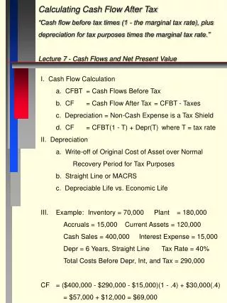
Calculating Cash Flow After Tax “Cash flow before tax times (1 - the marginal tax rate), plus depreciation for tax purposes times the marginal tax rate.” Lecture 7 - Cash Flows and Net Present Value I. Cash Flow Calculation a. CFBT = Cash Flows Before Tax b. CF = Cash Flow After Tax = CFBT - Taxes c. Depreciation = Non-Cash Expense is a Tax Shield d. CF = CFBT(1 - T) + Depr(T) where T = tax rate II. Depreciation a. Write-off of Original Cost of Asset over Normal Recovery Period for Tax Purposes b. Straight Line or MACRS c. Depreciable Life vs. Economic Life III. Example: Inventory = 70,000 Plant = 180,000 Accruals = 15,000 Current Assets = 120,000 Cash Sales = 400,000 Interest Expense = 15,000 Depr = 6 Years, Straight Line Tax Rate = 40% Total Costs Before Depr, Int, and Tax = 290,000 CF = ($400,000 - $290,000 - $15,000)(1 - .4) + $30,000(.4) = $57,000 + $12,000 = $69,000
Initial, Operating, and Terminal Cash Flows for an Expansion Project “Initial = Outflow Associated with Initial Investment, Operating = Occur Over Economic Life of a Project, and Terminal = Net Inflow or Outflow When Project Ends” Lecture 7 - Cash Flows and Net Present Value • 0 1 2 3 4 5 • I. |----------|----------|---------|----------|---------| • Init. Invest. Operating Cash Flows Terminal Cash Flow • II. INITIAL COSTS - AT t=0 • Plant, equipment, land purchased • Opportunity costs of land, etc. (owned but could be sold). • Transportation, installation costs of new plant/equipment • Additional working capital=Cur. Assets - Cur. Liabilities. • III. OPERATING CASH FLOWS • (Cash in - Cash out)(1 - T) + Depr(T) • We consider the asset's FULL economic life which is generally longer than its depreciable life => tax shield only in first few years. • If the acceptance of the project reduces cash flows from other projects this opportunity cost must be factored in, e. g., rent lost on floor space. • QUESTION: Suppose the building was not being rented?
Lecture 7 - Cash Flows and Net Present Value • IV. TERMINAL CASH FLOWS • Salvage value from asset sale = After-Tax Salvage • = Sale Price - (Sale Price - Book Value)(Tax Rate). • Where Book Value is the asset’s remaining depreciation. • Tax shield from loss due to asset sale - firm must be profitable. • Recapture of Net Working Capital • Cost of disposal of asset - strip-mine, nuclear plant (has been underestimated). • Tax liability due to sale of asset at a gain. • Example: • Suppose we have purchased a machine at $1.0M, with a depreciable life of 3 years, we use straight line depreciation, the tax rate is 40%, it produces revenues of $400,000 per year and variable expenses of $300,000 per year, and we can sell it for $100,000 at the end of 5 years. Show initial investment, operating and terminal cash flows.
Lecture 7 - Cash Flows and Net Present Value Initial = $1,000,000 at Time 0 Operating CF - Years 1 - 3 = ($400,000 - $300,000)(.6) + $333,333(.4) = $60,000 + 133,333 = $193,333 Operating CF - Years 4 - 5 = ($400,000 - $300,000)(.6) = $60,000 Terminal CF - Year 5 Salvage = $100,000(.6) = $60,000 Summary Year 0 = - $1,000,000 Year 1 = $ 193,333 Year 2 = $ 193,333 Year 3 = $ 193,333 Year 4 = $ 60,000 Year 5 = $ 120,000 Question: Is this a good corporate investment?
Initial, Operating, and Terminal Cash Flows for a Replacement Project “Unlike an Expansion Project - a Replacement Project Must Consider the Cash Flows Forgone By Replacing the Old Equipment, i.e., Incremental (new - old) Cash Flows.” Lecture 7 - Cash Flows and Net Present Value • ESTIMATING INCREMENTAL CASH FLOWS. • A. Incremental Initial investment DCF0 • Same • Equipment cost, transport costs, in working capital compared to old project, opportunity cost. • New • Inflow of funds from old asset sale including disposal costs (+) • Tax benefit (liability) on sale of old asset (+/-) • B. Operating Cash Flow • Incremental operating CF = CF • = (CFBTnew - CFBTold)(1 - T) + (Deprnew - Deprold)(T) • Just the difference between new and old cash flows and depreciation.
Lecture 7 - Cash Flows and Net Present Value • C. Terminal Cash Flow • Same • CF on new asset sale (+) • Tax benefit (liability) if asset sold at loss/gain (+/-) • Recapture all net working capital (+) • Disposal costs of new asset (-) • New • Funds that would inflow if old asset were sold (-) • Disposal costs that would have been paid on old asset (+) • Tax benefit (liab.) on replaced asset if it would have been sold for a loss (gain) (-,+) • ESSENTIAL DIFFERENCES • 1. Old asset is sold early - immediate inflow, disposal & tax • consequences (*Big Benefit-> May get tax benefit since • market value may be less than book value; eg. computers.) • 2. Old asset is not sold later - opportunity costs, disposal • and tax consequences. Examples include asbestos and • asphalt shingles - cost more to dispose later. • 3. Any effect on present and continuing investments. • 4. Forgone operating cash flows from replaced investment
Lecture 7 - Cash Flows and Net Present Value Example: E Services is considering replacement of a machine that was purchased 3 years ago for $60,000 and is generating CFBT of $15,000 per year. The machine’s depreciation is 5-year straight-line. If sold today it would bring $18,000; sold in 5 more years it would bring $10,000. The new machine would cost $75,000, be depreciated over 5 years with straight-line, require $8,000 in installation costs which will be expensed immediately, and generate $30,000 in CFBT. Its resale value in 5 years is $20,000. If E services’ tax rate is 40 percent and its cost of capital is 14 percent, should the machine be replaced? Calculate Incremental After-Tax CF’s Initial Investment Cost of new machine $75,000 Installation ($8,000)(1 - .40) 4,800 Old machine sale (18,000) Tax Saving from old’s sale (2,400) [$60,000 - (60,000/5)(3) - $18,000](.40) $59,400 Incremental Operating CF’s CF1-2 = (30,000 - 15,000)(1-.40) + (15,000 - 12,000)(.40) = 10,200 CF3-5 = (30,000 - 15,000)(1 - .40) + (15,000)(.40) = 15,000
Lecture 7 - Cash Flows and Net Present Value Terminal CF After-tax CF on sale of new machine (20,000 - 0)(.60) 12,000 minus the foregone After-tax CF on sale of old machine (10,000 - 0)(.60) (6,000) 6,000 NPV = -59,400 + 10,200[PVA.14,2] +15,000[PVA.14,3][PV.14,2] + 6,000[PV.14,5] = -12,704 Do Not Replace
Lecture 7 - Cash Flows and Net Present Value • Complications in Capital Budgeting • Incremental cash flows when replacing an asset or considering an asset that may impact profitability of other assets. • Shorter life cycles and more frequent replacement decisions. • Replacement Project <--------|--------> New Related Project (pure substitute) (independent) (pure compliment) • Risk adjustment to the discount rate for different risk projects. • Different discount rate for different parts of a single project.
Complimentary and Substitute Projects “A Complementary Project Increases Other Projects Cash Flows While a Substitute Project Reduces Other Projects. Lecture 7 - Cash Flows and Net Present Value Whenever a new project is accepted, in order to judge its merits properly, we must consider the positive or negative impact it has on the projects we already have or plan to accept. Example: T Products has two projects it may undertake. Project 1 produces Hawiian shirts and requires an initial investment of $150,000 and provides CFs of $60,000, $80,000 and $100,000 in years 1, 2, and 3 respectively.Project 2 produces Jamaican shirts and requires an initial investment of $60,000 and provides CFs of $30,000, $30,000 and $30,000 in years 1, 2, and 3 respectively. If both 1 and 2 are undertaken then project 1’s CF’s will be reducedby $10,000 per year. If the cost of capital is 14 percent, what should T Products do? NPVonly 1 = -150,000 + 60,000[PV.14,1] + 80,000[PV.14,2] + = 31,640 100,000[PV.14,3] NPVonly 2 = -60,000 + 30,000[PVA.14,3] = 9,660 NPV1 and 2 = 31,640 + 9,660 - 10,000[PVA.14,3] = 18,080 Just do project 1 alone.
Risk and Capital Budgeting “Various Methods to Handle Projects with Different Risk: CAPM and RADR” Lecture 7 - Cash Flows and Net Present Value 1. CAPM Method - assign project a beta and use k = kf + B(km - kf) 2. Risk-Adjusted Discount Rate (RADR) Method (Also Called Expected NPV Approach) Risk Adj. NPV = -E(CF0) + Here, E() means Expectation. We need to attach probabilities to possible CFs and find expected CFs. One Way to get RADR a. Calculate the Coefficient of Variation for CFs where CV = Standard Deviation of CFs / E(CFs) b. Start with MCC (Marginal Cost of Capital) Then Adjust MCC as follows RADR = MCC + Risk Adjustment (positive, zero negative) By Project Type Cost Reduction = Low Risk (small CV) -> adjust down Replacement Projects = Average Risk (average CV) -> no New Projects = High Risk (large CV) -> adjust up
Risk and Capital Budgeting “Various Methods to Handle Projects with Different Risk: Sequential Analysis” Lecture 7 - Cash Flows and Net Present Value Sequential Analysis to Adjust for Different Risks at Different Project Stages => Success => Large CF’s Research and => Sell in Test Market Build Prototype =>Failure => zero/Small CFs Use a large k for early risky stages and a smaller k for later, less risky stages. Similar to options analysis covered later. Steps: a. Get NPVs for Branches Using Small k b. Apply Probabilities to Each Branch NPV and Sum to Get Expected NPV c. Discount the Expected NPV Back to Time 0 Using Large k d. Discount Other Cash Flows From Earlier Periods in First Stage at Large k
Risk and Capital Budgeting “Sequential Analysis Continued” Lecture 7 - Cash Flows and Net Present Value II. Example: Suppose you have a project that requires an initial investment of $400,000 and $400,000 at the end of this year and next year for research. The required return for this research phase of the project is 30%. The projects second marketing phase will be a success with 75% probability or a failure with 25% probability. If a success, you will invest another $500,000 at the end of year 3 and receive $1,000,000 at the end of each of the next 4 years. If a failure, you will invest $200,000 at the end of year 3 and receive $200,000 at the end of each of the next 4 years. If the required rate of return for the second phase is 10%, should you make the investment? NPVsuccess = $1,000,000[PVA.10,4]-$500,000 = $1,000,000(3.170) - $500,000 = $2,670,000 NPVfailure = $ 200,000[PVA.10,4]-$200,000 = $ 200,000(3.170) - $200,000 = $ 434,000 Exp. NPV = .75($2,670,000) + .25($434,000) = $2,111,000 NPVoverall = -$400,000 - $400,000[PVA.30,2] + $2,111,000[PV.30,3] = $16,476 Decision: Accept.
Risk and Capital Budgeting “Various Methods to Handle Projects with Different Risk: Sensitivity Analysis and Break-Even Analysis” Lecture 7 - Cash Flows and Net Present Value SENSITIVITY ANALYSIS Vary some assumptions about the economy or industry (say oil prices) and find the effects on CFs and NPVs This is a way to force one to consider possible problems but is not an accurate method. Simulation - more complex sensitivity analysis - more variables change at once, random number generator chooses, results given as probability distribution, --> difference is that interdependency between changing variables can be handled easier. BREAK EVEN ANALYSIS IN A FINANCE (NPV=0) SENSE, NOT AN ACCOUNTING (DOLLAR) SENSE -> (EAT= 0) STEPS 1. Find CF annuity required to get NPV = 0 PVout = PVin Initial Investment = CF(PVAk,n) Initial Inv/(PVAk,n) = CF (break even cash flow)
Risk and Capital Budgeting “Various Methods to Handle Projects with Different Risk: Break-Even Analysis” Lecture 7 - Cash Flows and Net Present Value 2. Now find sales need to get CF Sales - (variable costs + fixed costs) - taxes = CF X - VX - F - (X - VX - F - Depr)(t) = CF where X = break even sales V = Variable cost as % of sales F = fixed cost t = Tax rate Depr = depreciation (actually a fixed cost) Compare to Accounting Break Even X - VX - F - Depr - (X - VX - F - Depr)(t) = 0 or X - VX - F - (X - VX - F - Depr)(t) = Depr Finance breakeven gets back present value of investment while accounting breakeven gets back dollars invested.
Risk and Capital Budgeting “Various Methods to Handle Projects with Different Risk: Break-Even Analysis” Lecture 7 - Cash Flows and Net Present Value Example: E Products plans a $4 million investment that will be depreciated over 10 years with straight-line. Variable costs are 50 percent of sales, fixed costs are $300,000 per year, the tax rate is 30 percent and the cost of capital is 18 percent. Find the accounting and financial break-even sales points and explain why they differ. Depreciation = 4,000,000/10 = 400,000 Accounting break-even X - .5X - 300,000 - 400,000 - (X - .5X -300,000 - 400,000)(.30) = 0 .35X -490,000 = 0 => X = 1,400,000 Financial break-even 4,000,000 = CF[PVA.18, 10] => CF = 4,000,000/4.494 = 890,076 X - .5X -300,000 - (X - .5X -300,000 - 400,000)(.30) = 890,076 .35X - 90,000 = 890,076 => X = 2,800,160 Financial breakeven is larger because it requires future cash flows to recover the present value of the investment.