Data Sources
320 likes | 447 Vues
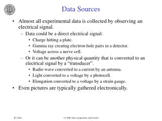
Data Sources. Almost all experimental data is collected by observing an electrical signal. Data could be a direct electrical signal: Charge hitting a plate. Gamma ray creating electron-hole pairs in a detector. Voltage across a nerve cell.

Data Sources
E N D
Presentation Transcript
Data Sources • Almost all experimental data is collected by observing an electrical signal. • Data could be a direct electrical signal: • Charge hitting a plate. • Gamma ray creating electron-hole pairs in a detector. • Voltage across a nerve cell. • Or it can be another physical quantity that is converted to an electrical signal by a “transducer”. • Radio wave converted to a current by an antenna. • Light converted to a voltage by a photocell. • Elongation converted to a voltage by a strain gauge. • Even pictures are typically gathered electronically. 111 BSC Data Acquisition and Control
Clean Signal: Signal Size Typical Data • Antimatter trap test: • Measurement: charge remaining in trap as a function of time. 111 BSC Data Acquisition and Control
Typical Data Complications: Coupling 111 BSC Data Acquisition and Control
Typical Data Complications: Jitter 111 BSC Data Acquisition and Control
Typical Data Complications: Filtering 111 BSC Data Acquisition and Control
Typical Data Complications: Coupling+Filtering+Jitter 111 BSC Data Acquisition and Control
Typical Data Complications: Coupling+Filtering+Jitter+Noise 111 BSC Data Acquisition and Control
Typical Data Complications: Coupling+Filtering+Jitter+Noise 111 BSC Data Acquisition and Control
Typical Data Complications: Extracted Signal Low Noise High Noise Live Analyze Data 10mV signal 111 BSC Data Acquisition and Control
Manual Data Acquisition • Little data is acquired manually: • Tedious. • Imprecise. • Error-ridden. • Limited data sets to small to perform sophisticated data analysis. 111 BSC Data Acquisition and Control
Data Acquisition • Data can be acquired by an instrument: Lock-In Amplifier Oscilloscope Data is then transmitted to a computer via a communication link: Ethernet, firewire, USB, serial, GPIB. 111 BSC Data Acquisition and Control
Instrument Computer Cable Controller Communications Standards: GPIB • The most common transmission standard is GPIB, also know as HP-IB and IEEE. See http://www.htbasic.com/support/tutgpib.html for a brief description of the standard. $500 $100 $500 More than one instrument can be run by the same controller. GPIB is expensive. 111 BSC Data Acquisition and Control
GPIB • GPIB is also: • Slow – 1.5Mbytes/sec. • Short Range – 2m maximum. • Difficult to use. • Archaic. So why do we use it? 111 BSC Data Acquisition and Control
Computerized Data Acquisition • Instead of using external instrumentation, we can use data acquisition cards installed directly into a computer. This card costs $675 ($1065 with cabling accessories), and acquires up to 250k samples/sec, on 16 channels, with 16bit accuracy. The card also has four 16bit analog output lines, and 48 digital lines. 111 BSC Data Acquisition and Control
Computerized Data Acquisition • Unlike standalone equipment, computer cards are worthless without decent interfaces. • Manufacturers provide a debugging interface. • Sometimes they provide a data logger. 111 BSC Data Acquisition and Control
Data Acquisition Environments • We want a data acquisition environment that is: • Flexible. • Powerful. • Easy to learn and use. • Self-documenting. • Doesn’t crash. • Efficiently uses computer resources. 111 BSC Data Acquisition and Control
Data Acquisition Environment: Excel • Addins allow excel to acquire data. • Very limited functionality. • Pathetic graphs. • Utterly undocumentable. • Inefficient. 111 BSC Data Acquisition and Control
Unjustifiably insufferable manufacturer. Data Acquisition Environment: Mathematica • Addins allow Mathematica to acquire data. Mathematica has: • Gorgeous graphs. • Powerful symbolic manipulation functions. Addins are shoe-horned in. Limited functionality. Obscure and difficult to learn. Inefficient. 111 BSC Data Acquisition and Control
Data Acquisition Environment: Matlab • Addins also allow Matlab to acquire data. Matlab has: • Powerful data analysis capability. • Good graphics. Addins are shoe-horned in. Limited functionality. Obscure and difficult to learn. Pathetic, 1970’s user interface. 111 BSC Data Acquisition and Control
Data Acquisition Environment: C • Most data acquisition cards can be called from C. • Primitive acquisition commands, but powerful. • Can be very efficient. • Difficult to use and learn. • Primitive or non-existent graphing capability. • Does not have built in analysis packages. • Can be documented, but rarely is… 111 BSC Data Acquisition and Control
Data Acquisition Environment: LabVIEW • LabVIEW is a quirky graphical programming language specifically designed for data acquisition, analysis, and control. It is: • Easy to learn and use. • Powerful and flexible. • Self-documenting. • Efficient. 111 BSC Data Acquisition and Control
LabVIEW • LabVIEW programming is similar to drawing flow charts. • LabVIEW programs consist of a Front Panel: 111 BSC Data Acquisition and Control
LabVIEW • and a Block Diagram: Data flows through the wires to the operators and subroutines. Data is input by controls, and output by indicators. 111 BSC Data Acquisition and Control
LabVIEW Example: Get Signal • Place and configure a DAQ Assistant Express vi. Configure as follows: • Input on AI7 (or some other channel.) Attach a 30cm diameter loop antenna to the input. • Sample rate to 1.6MHz. [This exceeds the maximum spec’d rate for our card (the PCI-MIO-16-4-E, now know as the PCI-6040E,) which is 500kHz. Nonetheless, the card still works at this rate.] • Sample size to 160k: i.e. a 0.1s second sample. • Input range to +-10mV. • Wire the output to a Graph Indicator. • Run the vi several times, demonstrating that the signal looks like noise. • Set to the time scale to 20uS, and turn off X autoscaling. Run several times to show the detailed shot-to-shot variations. • To exhibit the quantization, change the plot type to “line with points.” (Do not show the entire data set while displaying the points; LabVIEW may hang for many seconds.) • Restore the plot type to “line” and turn on autoscaling. 111 BSC Data Acquisition and Control
LabVIEW Example: Signal Spectrum Disconnect the Graph and route the signal to Spectral Measurements Express vi. Configure the vi to display in dB. Route the output of the Spectral Measurements vi to the Graph. Run the vi repetitively, showing both the noise and the repeatable peaks. Set to the Frequency scale to 1kHz, and turn off X autoscaling. Run repetitatively. What are the peaks? Set the Frequency scale to 500kHz-800kHz. What are the peaks? Look at one peak closely: for instance, change the scale to 605kHz-615kHz. Change the Spectral Measurements Express vi to output linear RMS Magnitude. How big is the signal? 111 BSC Data Acquisition and Control
LabVIEW Example: Filtered Signal Disconnect the Graph and delete the Spectral Measurements Express vi. Add a Filter Express vi. Configure the filter to be a bandpass around one of the peaks previous identified, for instance between 605kHz and 615kHz. Route the output of the DAQ Assistant Express vi to the original Graph. Wire the filtered signal to a new Graph. Change the time scale on both graphs to 10ms, turn off autoscaling, and run repetitively. Compare the filtered to the unfiltered signal. Is the filtered signal recognizable? Also try a timescale of 1ms. 111 BSC Data Acquisition and Control
LabVIEW Example: Demodulating AM • An AM signal is an amplitude modulated carrier wave. 111 BSC Data Acquisition and Control
LabVIEW Example: Demodulating AM 111 BSC Data Acquisition and Control
LabVIEW Example: Partially Demodulated RF Signal Add an absolute value operator after the filter to demodulate the RF. Run repetitively, and watch the output. 111 BSC Data Acquisition and Control
LabVIEW Example: Fully Demodulated RF Signal Add a Filter Express vi after the absolute value. Configure the bandpass filter to 100Hz-3kHz. Run repetitively, and watch the output. 111 BSC Data Acquisition and Control
LabVIEW Example: Convert to Audio The signal from the filter is sampled at 1.5MS/s. The audio card requires a much slower sample rate: 11025S/s. Decimate the signal using the Align and Resample Express vi. Configure the vi to a “Specific dt” of 1/11025=9.07E-5s. Multiply the resulting signal by 200E6. Wire this signal into the “mono 16-bit” input of the Snd Write Waveform vi. Create a constant for the “sound format,” and change from “8 bit” to “16 bit.” Change the DAQ Assistant vi to acquire 2.4M points. Run repetitively, turn on the sound, and watch the output. 111 BSC Data Acquisition and Control
LabVIEW Example: AM Software Radio The previous example plays 1.5s snippets. Modifying the program to play continuously is a bit complicated. Both the RF signal and the audio signal needs buffering. The program AM Software Radio.vi implements the required buffering 111 BSC Data Acquisition and Control