Download
1 / 31
310 likes | 335 Vues
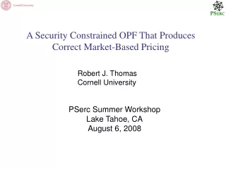
A Security Constrained OPF That Produces Correct Market-Based Pricing. Robert J. Thomas Cornell University. PSerc Summer Workshop Lake Tahoe, CA August 6, 2008. Contributors to the “SuperOPF”. Alberto Lamadrid Carlos Murillo-Sánchez Robert Thomas Zhifang Wang Hongye Wang Ray Zimmerman.

E N D
A Security Constrained OPF That Produces Correct Market-Based Pricing Robert J. Thomas Cornell University • PSerc Summer Workshop • Lake Tahoe, CA • August 6, 2008
Contributors to the “SuperOPF” • Alberto Lamadrid • Carlos Murillo-Sánchez • Robert Thomas • Zhifang Wang • Hongye Wang • Ray Zimmerman
Why a SuperOPF? • State of the art for planning & real-time operations is primitive w.r.t. ancillary services & pricing needed to support market design. • Tools are needed to capture true value of resources, e.g. demand response and uncertain energy sources. • Proper allocation and valuation of resources requires true simultaneous co-optimization.
What is the SuperOPF? Computational Complexity is an Issue!
Simple Example of Sequential OPF System Parameters • Generators • 1: [0,400] MW, $25/MWh, 10MW/min • 2: [0,300] MW, $30/MWh, 10MW/min • 3: [0,200] MW, $80/MWh, 15MW/min (Unavailable) • Lines: All X=0.01 • 1-3: [-240,240] MW • 1-2: [-300,300] MW • 2-3: [-300,300] MW • Load: 450MW, 175 MW is shed-able. VOLL=$5,000/MWh • Contingencies • Loss of line 1-2 • Loss of largest generating unit - Gen1
Simple Example [0,400] MW $25/MWh, 10MW/min [0,300] MW, $30/MWh, 10MW/min Dispatch Cost - $12,150 Unavailable Unconstrained Dispatch Cost = $11,250 This is the OPF dispatch that would occur if line limits were included but contingencies are not. Call this the no-contingency dispatch (NCD). This configuration is unreliable with respect to contingencies.
A feasible dispatch arrived at through sequential optimization Dispatch Cost - $12,300 In this configuration, an outage of line 1-2 would produce a flow on line 1-3 of 240MW’s. An outage of Gen 1 would require a load shed of 150MW’s and a ramp of Gen 2 to 300 MW which it could do in 9 minutes.. But this dispatch does not take advantage of Gen 1’s ramping capability.
The least-cost reliable intact system dispatch produced by the SuperOPF Dispatch Cost - $12,250 In this configuration if the line contingency occurs Gen 1 would have to back off 10 MW and Gen 2 would have to ramp up 10 MW to avoid overloading line 1-3. If Gen 1 is outaged then Gen 2 would have to ramp up 100 MW to its 300MW limit and 150 MW’s of load would have to be shed.
Problems included in the formulation • standard OPF with full AC non-linear network model and constraints • n–1 contingency security with static and dynamic constraints • procurement of adequate supply of active and reactive energy and geographically distributed reserves
uncertainty of demand, wind, contingencies • stochastic cost, including cost of post-contingency states • correct prices for day-ahead contracts for energy, reactive supply and reserve • consistent mechanism for subsequent re-dispatching and pricing, given specific realization of uncertain quantities
Problems not yet included • thermal / hydro unit commitment • We have a formulation that could be included at a later stage. • transient upset following contingencies • Only included in the the form of angle difference limits.
Conceptual Framework • Replicate network for multiple scenarios. • Treat as single large network with islands. • All standard OPF variables for all islands are available to impose costs & constraints. • Additional variables can be defined and included in costs and linear constraints. • Additional linear constraints on all variables
Day-ahead Market • Scenarios include projected base case plus set of credible post-contingency cases. • All standard limits (voltage, flow, etc.) apply to base case and post-contingency cases. • Standard OPF cost function on active and reactive output included for base case and post-contingency cases, weighted by probabilities.
Additional variables include: • day-ahead contracted energy allocation • positive & negative post-contingency deviations from day-ahead contract • reserve quantities (max of these deviations) • Additional costs include: • probability weighted cost of deviations from contract • cost of reserves
Additional constraints include: • limits on reserve quantities • physical ramp rate limits on deviations of post-contingency output from base case output
Real-time Re-dispatch • Same as day-ahead, except: • Updated demand forecasts, outages, credible contingency list, probabilities, etc. • Day-ahead contracted quantity is now fixed. • Reserve quantities are now fixed limits.
Determining the Economic Benefits of Avoiding Loss-of-Load during Contingencies: A Case Study • Area 1 • Urban • High Load • High Cost • VOLL = • $10,000/MWh • Area 2 • Rural • Low Load • Low Cost • VOLL = • $5,000/MWh • Area 3 • Rural • Low Load • Low Cost • VOLL = • $5,000/MWh
The Underlying Rationale for Doing this Case Study • Region 1 represents an urban load pocket with high load, high cost generation, and high VOLL. • Regions 2 and 3 represent rural areas with low load, low cost generation, and low VOLL. • Transmission capacity into Region 1 from Regions 2 and 3 is relatively limited. • An economic dispatch would use generation in Regions 2 and 3 as much as possible and use generating capacity in Region 1 for reserves to maintain operating reliability (e.g. guard against line outages). • In this Case Study, operating costs remain constant, offers equal the true marginal costs, and all loads in Region 1 are increased in increments until things start to go wrong (i.e. load outages occur).
The Basic Objective Function Subject to meeting LOAD and all of the nonlinear AC CONSTRAINTS of the network Where k is a CONTINGENCY i is a GENERATOR j is a LOAD CG(Gi) is the COST of generating G MWh CR(Ri) is the COST of providing R MW of RESERVES VOLLj is the VALUE OF LOST LOAD LNS(G, R)j is the LOAD NOT SERVED
Contingencies Considered • Number Probability • 0 = base case 95% • 1 = line 1 : 1-2 (between gens 1 and 2, within area 1) 0.2% • 2 = line 2 : 1-3 (from gen 1, within area 1) 0.2% • 3 = line 3 : 2-4 (from gen 2, within area 1) 0.2% • 4 = line 5 : 2-5 (from gen 2, within area 1) 0.2% • 5 = line 6 : 2-6 (from gen 2, within area 1) 0.2% • 6 = line 36 : 27-28 (main tie from area 3 to area 1) 0.2% • 7 = line 15 : 4-12 (main tie from area 2 to area 1) 0.2% • 8 = line 12 : 6-10 (other tie from area 3 to area 1) 0.2% • 9 = line 14 : 9-10 (other tie from area 3 to area 1) 0.2% • 10 = gen 1 0.2% • 11 = gen 2 0.2% • 12 = gen 3 0.2% • 13 = gen 4 0.2% • 14 = gen 5 0.2% • 15 = gen 6 0.2% • 16 = 10% increase in load 1.0% • 17 = 10% decrease in load 1.0%
Expected Nodal Prices for GeneratorsPrice Differences are Caused by Congestion $90/MWh $20/MWh Higher Load in the Load Pocket (Region 1) ->
Expected Nodal Prices for LoadsThe Large Price Differences Within Area 1 (blue) are Caused by Load Shedding --- A Very Localized Effect $10,000/MWh $10/MWh Higher Load in the Load Pocket (Region 1) ->
The Expected Cost of Lost Load(Weighted by the Probability of Each Contingency) $4,500/MWh Contingency Higher Load in the Load Pocket (Area 1) -> Problems show up first in contingencies as system load increases
The Shadow Price of the Flow on Tie Line 15 Linking Areas 2 and 3 by Contingency $80/MWh Contingency Higher Load in the Load Pocket (Area 1) -> Typical Example of Binding Flow Limits on Power Transfers
The Shadow Price of the Flow on Line 10 in Area 1 by Contingency $10,000/MWh Choose Scale Factor = 1.1278 for next part of the analysis (System Load = 200MW) Contingency Higher Load in the Load Pocket (Area 1) -> Caused by a Binding Flow Limit WITHIN Area 1 --- Like NYC?
The Question for Planners I: Will it Pay to Increase the Capacity of Line 10? STEP 1 STEPS • Specify the Hourly Loads for a Year. • Specify a Peak Load of 200MW (when load shedding first occurs in some contingencies). • Determine the Nodal Prices, Revenues and Costs • Compute the Annual Totals
STEPS 2 and 3 Low Load - base system High Load - base system Load Shedding AND Congestion (i.e. High Prices) only occur for a Few Hours. Most of the time Loads pay the True Marginal Cost of Energy. Net Revenues for Baseload Units are Large --- Where do the $$$ go? Low Load - Transmission improvement High Load - Transmission improvement Transmission Improvement => line 6-8 capacity doubled
The Question for Planners III: Will it Pay to Increase the Capacity of Line 10? STEP 4
Conclusions • A large part of the economic benefit of adding equipment to the network may be avoiding LOSS OF LOAD when credible contingencies occur (e.g. N-1 contingencies). • By using the SuperOPF, it is possible to identify the LOCATION of weaknesses on the network and the net economic benefit of upgrading the network. • The same analytical framework can be used for PLANNING purposes, and problems tend to occur first when contingencies occur in a simulation (e.g. when load outages occur and violate standards of operating reliability). • GET THE PRICES RIGHT BY MAKING CONTINGENCIES EXPLICIT AND USING AN AC NETWORK FOR PLANNING.