GENERALIZED DISTANCE TRANSFORM
GENERALIZED DISTANCE TRANSFORM. A linear time algorithm and its application in fitting articulated body models. OUTLINE. Distance Transform Generalized Distance Transform Linear time algorithm for Euclidean distance Other distances Application of GDT

GENERALIZED DISTANCE TRANSFORM
E N D
Presentation Transcript
GENERALIZED DISTANCE TRANSFORM A linear time algorithm and its application in fitting articulated body models
OUTLINE • Distance Transform • Generalized Distance Transform • Linear time algorithm for Euclidean distance • Other distances • Application of GDT • Efficient matching of articulated body models
DISTANCE TRANSFORM Defined for a set of points P on a grid G, with P a subset of G G p q
EXAMPLE Example: G p q
EXAMPLES • Chamfer • Hausdorff • Hough • Often used in binary (edge) image matching
GENERALIZED DISTANCE TRANSFORM Instead of binary indicator function 1(q), we can assign a “soft” membership of all grid elements to P f(q) is sampled on the grid G f(q) does not have to be a 2D image, it can represent any D-dimensional, discrete space that encodes spatial relationships through d(p,q)
APPLICATIONS OF GDT • Feature matching / tracking • f(q) can represent a D-dimensional feature vector at location q, and d(p,q) is a displacement in the image space • Dynamic Programming / stereo matching • f(q) can represent the accumulated cost of coming to state p, and d(p,q) is a transition cost to move from state p to state qf’(q) = b(q) + minp(f(p) + d(p,q)) • Belief Propagation / MRFs • Max product (negative log) m’ji(xi) = minxj(’j(xj) + ’ji(xj-xi) + kN(j)\im’kj(xj))
WHY SO SLOW? • Generalized DT computes for each grid point p the distance to all other grid points q • Its complexity is O(n*n) in the number of grid locations n • Intractable for problems with large number of discrete locations
MIN CONVOLUTION Speed-up by seeing DT as Min-Convolution
f(q) f(2) f(1) f(3) f(0) 0 1 2 3 q LOWER ENVELOPE f(q) • Min Convolution is the Lower Envelop of cones placed at each p • Example 1 • One Dimension • Euclidean Distance 0 1 2 3 q Remember: in the case of standard distance transforms all cones would either be rooted at zero (when there is a pixel) or at infinity (when there is no pixel)
LOWER ENVELOPE • Example 2 • One Dimension • Squared Euclidean • Once computed, the distance transform on the grid can be sampled from the lower envelope in linear time
COMPUTING THE LOWER ENVELOPE Add parabola at first grid point q
COMPUTING THE LOWER ENVELOPE Add second parabola at second grid point, and compute intersection with previous parabola v[1] q s
COMPUTING THE LOWER ENVELOPE Insert height and intersection point in arrays v and z v[1] v[2] z[2]
COMPUTING THE LOWER ENVELOPE Add third parabola at third grid point, and compute intersection with previous parabola v[1] v[2] q z[2] s
COMPUTING THE LOWER ENVELOPE Since the new intersection is to the right of the previous intersection, insert height and intersection point in arrays v and z v[1] v[2] v[3] z[2] z[3]
COMPUTING THE LOWER ENVELOPE Now consider the case when the new intersection is to the left of the previous intersection v[1] v[2] q s z[2]
COMPUTING THE LOWER ENVELOPE Delete previous parabola and its intersection from arrays v and z and compute intersection with the last parabola in array v v[1] q s
COMPUTING THE LOWER ENVELOPE Now insert height and intersection point in arrays v and z v[1] v[2] z[2]
COMPUTATIONAL COMPLEXITY • The algorithm has two steps • 1) Compute Lower Envelope • For each grid location: • One insertion for parabola and intersection point • At most one deletion of parabola and intersection point • Hence, O(n) for n grid locations • 2) Sample from Lower Envelope • O(n) So, total complexity of O(n) !
ARBITRARY DIMENSIONS • Consider 2D grid: • Any d-dimensional DT can be performed as d one-dimensional distance transforms in O(dn) time is the one-dimensional DT along the column indexed by x’
OTHER DISTANCES • So far only Euclidean distances shown • Other distances realized as a combination of linear, quadratic and box distances • Min of any constant number of linear and quadratic functions, with or without truncation • E.g., multiple “segments” • Gaussian approximation with four min convolutions using box distances
ILLUSTRATIVE RESULTS Borrowed from Dan Huttenlocher • Image restoration using MRF formulation with truncated quadratic clique potentials • Simply not practical with conventional techniques, message updates 2562 • Fast quadratic min convolution technique makes feasible • A multi-grid technique can speed up further • Powerful formulationlargely abandonedfor such problems
Illustrative Results Borrowed from Dan Huttenlocher • Pose detection and object recognition • Sites are parts of an articulated object such as limbs of a person • Labels are locations of each part in the image • Millions of labels, conventional quadratic time methods do not apply • Compatibilities are spring-like
best configuration match cost deformation cost THE GENERAL APPROACH • Body parts model appearance • Graph models deformation of linked limbs G=(V,E) with V set of part vertices, E set of edges connecting vertices • The best fit minimizes the sum of match cost of each limb and deformation cost of body structure
DYNAMIC PROGRAMMING • If Graph has tree-structure we can reformulate in recursive form -> Dynamic Programming (DP) • DP is appealing because it gives a global solution (on a discretized search space) • However, DP runs in polynomial time O(h2n), with n the number of parts and h the number of possible locations for each part • h usually is huge, often hundreds of thousands (x,y,s,θ) If each of (x,y,s,θ) has 20 discreet states, then we have h=160000 !!!
DP FOR TREE-STRUCTURED MODELS • Match quality for leaf nodes • Match quality for other nodes • Best location for root node
Need to transform lj into regular grid for which dij serves as distance measure MATCH COST AS DISTANCE TRANSFORM • Recall Generalized Distance Transform • Compare to match cost function
ORIGINAL BODY CONFIGURATION • Locations of two connected parts • Joint probability of both parts given deformation constraints
TRANSFORMED BODY CONFIGURATION • Project distribution over angles onto 2D unit vector representation • Now all parameters are in a grid and modeled as multivariate Gaussian with zero mean and variances specified in diagonal covariance matrix Dij • Distance in grid is given as Mahalanobis distance Dij over transformed joint locations Tij(li) and Tji(lj)
SUMMARY • Now linear instead of quadratic time to compute match costs between child and parent limbs • Did not prune away search space (still global solution!) • Search space only got a little bigger (about four times) due to unit vector representation of limb orientation • 32 discreet angles represented in 11x11 grid
REFERENCES • Daniel Huttenlocher • http://www.cs.cornell.edu/~dph/ • Pedro Felzenszwalb • http://people.cs.uchicago.edu/~pff/ • Distance Transforms of Sampled Functions. Pedro F. Felzenszwalb and Daniel P. Huttenlocher. Cornell Computing and Information Science TR2004-1963. • Pictorial Structures for Object Recognition, Intl. Journal of Computer Vision, 61(1), pp. 55-79, January 2005 (Daniel P. Huttenlocher, P. Felzenszwalb).
OTHER REFERENCES • Stereo & Image Restoration • Efficient Belief Propagation for Early Vision.Pedro F. Felzenszwalb and Daniel P. Huttenlocher. International Journal of Computer Vision, Vol. 70, No. 1, October 2006. • Higher Order Markov Random Fields • Efficient Belief Propagation with Learned Higher-Order Markov Random Fields, Proceedings of ECCV, 2006 (D. Huttenlocher, X. Lan, S. Roth and M. Black). • www.cs.ubc.ca/~nando/nipsfast/slides/dt-nips04.pdf • Image Segmentation • Efficient Graph-Based Image Segmentation. Pedro F. Felzenszwalb and Daniel P. Huttenlocher. International Journal of Computer Vision, Volume 59, Number 2, September 2004.
MATCH COST AS DISTANCE TRANSFORM • Distance p(x,y) in grid is given as Mahalanobis distance Mij over model deformation parameters lj=(x,y,s,θ)T